7 Model-Based Development and Use of a CNC Milling Machine
7.1 Chapter Introduction
CNC Milling Machines are at the heart of our manufacturing economy. In fact, GCode was originally developed for their use before being extended to other processes like 3D Printing (Section 1.2.1). We use them to make aircraft parts, car parts, moulds and all manner of tooling, surgery robots, spacecraft, gearboxes in wind turbines, scientific instruments, the list is endless. Perhaps most relevant for readers of this thesis: CNC Mills are often called mother machines; they are where we start when we want to build more machines.
Note that while “CNC” stands just for Computer Numeric Control and technically i.e. a 3D Printer is a CNC Tool, in practice we often simply use CNC to mean CNC Machining.
- A major issue facing the manufacturing economy today is that training new CNC Operators (aka CNC Programmers) takes too long (up to three years). In contries without good trades education (i.e. the US), there is a dearth of operators. Cite: 1m high paying mfg jobs go unfilled in the US every year.
- Understanding what will and won’t work in a CNC Toolpath is especially hampered by the hidden optimization (Section 1.2.4.1): cutting physics is particularely sensitive to changes in translational rates due to machine acceleration.
- Designing CNC Machines remains an art; actual machine performance is the result of interactions between motors, machine physics, and controllers themselves. This might limit the rate at which new CNC firms enter the market, or the rate at which existing firms develop new models.
7.1.1 Methods and Evaluation Overview
Many parts of this thesis revolve around the idea that we can formulate machine control as a constrained optimization problem. Model building is a prerequisite for machine controllers that are explicitly framed as constrained optimization solvers, and I demonstrated how these can be developed for motion control (Chapter 5) and for process and motion control as a coupled problem (Chapter 6). I also discussed how models can be used as tools for machine users, enabling them to more easily operate and understand their machines (Section 6.11.1 and Section 6.11.2) and their materials (Section 6.11.3). In this chapter, I will explore the use of models within human-in-the-loop design and operation workflows.
This will take up a few connected sections.
First, I will cover the basics of machining physics in Section 7.2.1, and explain the state of the art workflow in Section 7.2.2. I will also discuss existing work in the development of models for CNC in Section 7.2.4. I will then explain my methods for model-based design of a CNC machine (Section 7.3), and model-based operation of the same (Section 7.4). In the results section, I will show how motor models were used to evaluate trade-offs in motor selection for a machine (Section 7.5.2), and look at machined components and data from this machine’s operation (Section 7.5.3). I will show how models and our unique control architecture can be used to expose the hidden optimization to machine programmers in Section 7.4.1. I will also assess the quality of our model fits against real world data in Section 7.5.5, and in Section 7.4.2 I will show how those models can be combined with real-world measurements to estimate cutting force data from motor data alone.
To close the chapter, I will share and discuss the results in Section 7.5, and look ahead to cutting force model buildling, chatter detection and correction, and what it might look like to take on CNC Machining as an explicit constrained optimization problem (Section 7.7).
7.2 Background in CNC Machining
7.2.1 CNC Physics
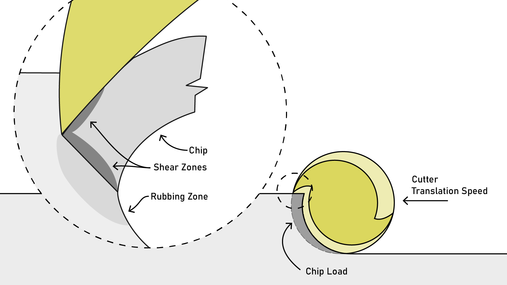
The physics of maching are arguably more intense than their counterparts in FFF, involving extreme shear rates, thermodynamics, tool life and geometry. The core of it is about chip load, which depends on the ratio between spindle RPM and translational velocity. Cutting an oversized chip will generate too much cutter force (leading to broken tools, a stalled spindle or actuator motor, or eggregious excitation of the machine or part’s resonance). Cutting an undersized chip (smaller than or close to size of the flute’s tip radius) means that the cutting physics become rubbing physics: this generates an exceptional amount of heat, dulls tools or leads to material buildup on the flute edge, and in some cases can weld the cutter and the part together which almost always leads to a machine crash.
Another important parameter is surface speed, which is the speed which the flute edge passes by the material being cut. It is a function of tool diameter and spindle RPM. Physically, this is related to the shear rate in the material as it is being separated from the work piece. Changes in shear rate affect chip formation: low shear rates tend to make larger chips (which can be difficult to evacuate from the work piece and can lead to “chip re-cutting”). Larger shear rates exert more total stress in the chip, leading it to break up into smaller chips that are more easily evacuated. The ideal shear rate for a cut is mostly a function of the material being cut and it’s temperature, but also of the tool geometry, sharpness and surface finish.
These physics all exert loads on the machine itself, it’s actuators, and the workpiece. Actuators must produce enough force to push the cutter through the piece, and spindle motors must produce enough torque to keep the tool rotating at the desired speed.
Most complex of all in CNC Machining is the issue of resonance: any machine has a given natural frequency and if chip formation happens to excite the machine near that frequency, the whole system vibrates, causing innaccuracies or even tool breakage.
7.2.2 The State of the Art CNC Workflow
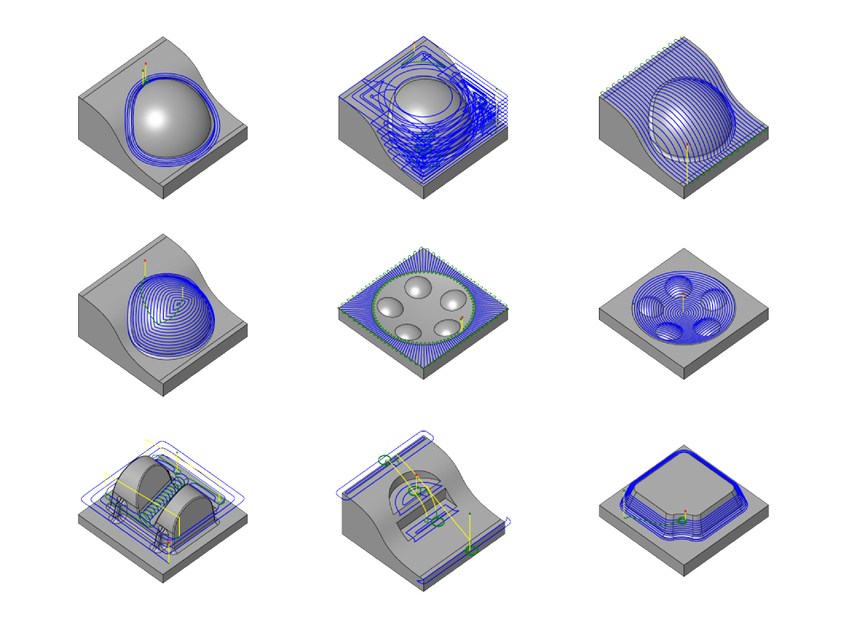
CAM for 3D Printing (aka ‘slicing,’ Section 6.2) is much simpler than CNC Machining because each job is effectively one operation: slice into layers, produce perimeters and then infill for each layer. That is, same basic geometric algorithms can be applied to just about every different part. A machining job can include many (tens or hundreds) of different path planning strategies for different geometric features, each selected manually. I show a selection of these strategies in Figure 7.3.
This also applies to tool selection. For example there is an obvious trade-off between large removal rates using big tools and detailed operations using smaller tools. There are also special cases; a tightly toleranced hole may require the machinist to select a purpose-made reaming tool, threaded features require threading tools, radiused or chamfered corners require fillet or chamfer end-mills, etc.
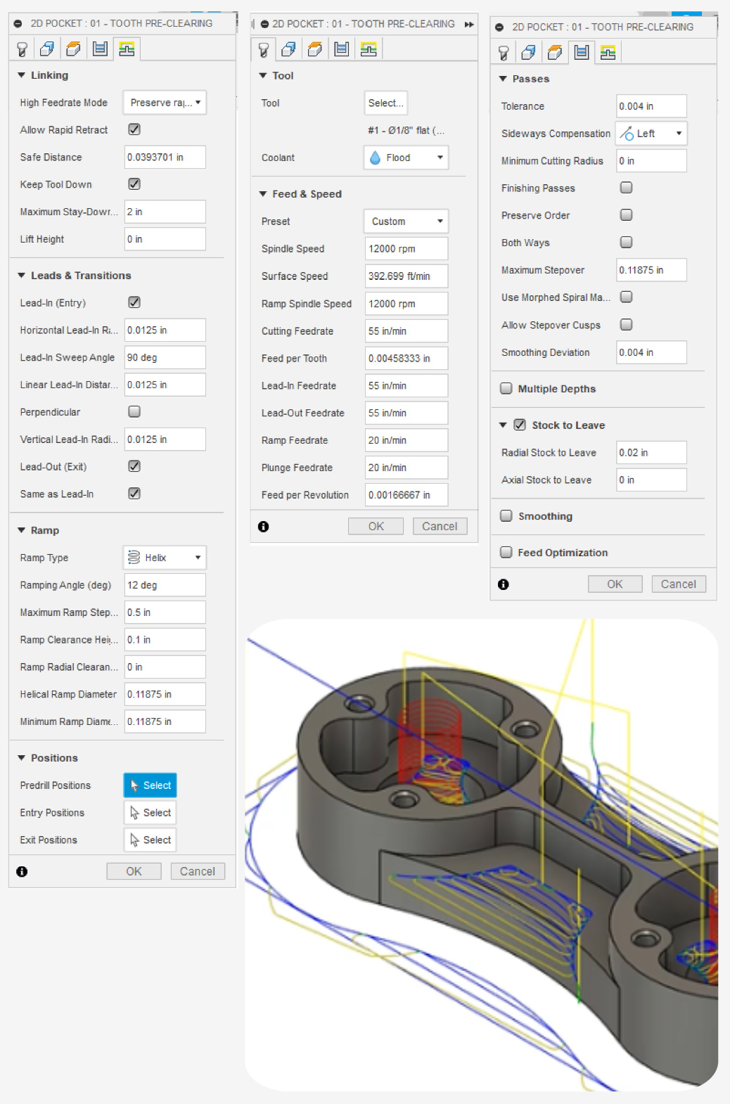
CNC CAM is similar to FFF Slicing where parameter selection is concerned. Once geometry and tools are selected, users must tune a littany of speed and cutting parameters. These define how fast the tool should move through the part, how much material should be cut with each pass (stepover and stepdown), and how fast the spindle should run. These are known colloquially as speeds and feeds and affect cutting physics in the ways mentioned above. Starter values for feeds and speeds can normally be calculated from tabulated values for surface speed and chip load, but even tabulated windows can be large and need to be heuristically tuned.
Milling parameters, then, are similar to FFF parameters: a user sets geometric and speed-related parameters that are only indirectly related to the underlying process physics that govern the system. Instead they are directly related to the low-level instructions (GCodes) that we send to the machine.
In all other ways, the state of the art CNC workflow is similar to FFF. Users import part geometry into a CAM package, configure geometric and low-level parameters, export GCodes, and run them on their machines. They watch the machine and listen to it, iterate on their parameters, and make incremental improvements to their selections using their own intuitions for the process and machine physics.
7.2.3 Interaction between Cutter Parameters and Acceleration Control
A key focus in this chapter will be the interaction between machine controllers and cutter parameters, namely chip load.
With CNC milling, deccelerating into a corner can change chip size dramatically. Machines need to slow down through corners to avoid violating their actuator constraints, but they manage to decelerate and accelerate at rates quite quickly. Spindles have very large rotational inertias, so we cannot rapidly slow them down to maintain chip load as the machine’s translational velocity changes. Instead, we simply have a lossy layer here. We may setup a job to run at a particular chip size, but tight corners in the job will done at much lower speeds with a much smaller chip size1. CNC Controllers don’t expose this acceleration control layer to users, and it is not specified in GCodes.
7.2.4 The State of the Art in Model-Based CNC
7.2.4.1 Estimating Cutting Force
While the physics that generate cutting forces are intense (high shear rates, plastic deformation, heat and mass flow, etc…), we only need to model those physics if we want to look at cutting forces in small length scales: i.e. understand chip formation and evacuation, tool life, etc. In our case, we just want to understand the loads seen by the machine. A former CBA undergraduate researcher Chetan (who I was able to help out!) wrote his thesis on the topic (Sharma et al. 2021), I was also able to find another masters’ dissertation: (Dunwoody 2010). Both outline relatively simple models that output radial and tangential cutting forces as a function of straightforward geometric parameters (cutter size, cut depth, spindle rpm and linear feedrate), with four coefficients to fit for cutting force and edge force coefficients, each with tangential and radial coefficient respectively.
\[ \begin{aligned} F_t = K_{tc}ah(\theta) + K_{te}a \\ F_r = K_{rc}ah(\theta) + K_{re}a \\ \\ a = \text{cut area} \\ h = \text{cut height} \\ \theta = \text{chip thickness} \\ K_{tc}, K_{rc} = \text{cut force coefficients} \\ K_{te}, K_{re} = \text{edge force coefficients} \\ \end{aligned} \tag{7.1}\]
(Sharma et al. 2021) shows that coefficients can be estimated using data generated on-machine, using measured spindle power and force exerted on the workpiece (a loadcell). In this work, I essentially replicate Chetan’s measurement setup, building a CNC machine with loadcells installed between each axis’ ball nut and carriage, and I chat over RS-485 to the machine’s spindle controller to measure spindle load.
7.2.4.2 Measuring Machine Stiffness and Resonance
In practice chatter causes more displacement than static loading. (Dunwoody 2010) adds resonance measurements: he uses a solenoid hammer to generate a step response of the tool, measuring the tools ‘ring’ using an inductive probe as a displacement sensor. Using this system, he generates a stability plot across spindle RPMs and depths of cut. In (Aslan and Altintas 2018), the authors develop a system that communicates with a Heidenhein machine controller at 10kHz to detect chatter in real-time using motor currents, and (Bort, Leonesio, and Bosetti 2016) develop a model-based adaptive controller to mitigate chatter and (Ward et al. 2021) implements a “machining digital twin” to optimize feedrates of a milling center in real-time to predict and automatically prevent chatter. Finally, for a broader overview of machining dynamics, we also have (Schmitz and Smith 2009) and (Altintaş and Budak 1995). I pass over this topic due to time (and, I should admit, skill issue) limitations, but show that our data contains enough information to characterize resonance.
7.3 Machine Design Tools
When we develop machines, we must select from discrete families of off-the-shelf parts with limited customization (especially if we are a small firm or individual with small order quantities). Of particular interest is motor selection, where we must consider characteristics of our motors and our machine’s kinematics since both affect the final performance.
For example, motor physics makes for natural trade-offs between availability of low- and high-end torque (Section 5.8.2). Motor parameters that help us understand these trade-offs are often often available from manufacturers, but not always, and as I discuss in 5.8.2 even two identical motors (same make and model) may have slightly different parameters. The most useful motor selection tool that is normally available from manufacturers is the motor torque curve (where we see how much force the motor can generate across a range of speeds), but torque curves can change depending on motor drive voltage and controller type.
It is also sometimes difficult to understand how motor torque curves might couple into a machine’s dynamics, through it’s drive system (belts, leadscrews, linkages, masses and frictions etc). At MIT, spreadsheets are the state-of-the-art design tool of choice for this step (n.d.). Spreadsheets are excellent design tools, but they tend to require that we iteratively step through dynamical states (acceleration, velocity) to understand performance, and require that we use multiple spreadsheets to understand each component of our machine. They also require that we input model parameters manually, and they are of course not complete simulation tools that can be subjected to virtual operation.
In this section, I develop tools that allow us to virtually swap motors onto simulated hardware to analyse machine performance across a range of parameters. We do this using both abstract parameter spaces and using real toolpaths. I discuss the use of these tools in 7.5.2.
7.3.1 Virtually Comparing Motor and Machine Dynamics
In Section 5.3.1, I showed how we can develop motor models using a closed-loop motor controller and simple test inertia. In Section 5.3.2, I showed how we can use those models to develop kinematic models of machines that include mass and damping terms.
Both of those models remain separable, which means that given a set of motor models and a machine’s kinematic model, we can virtually compare performance across motor options.
![]()
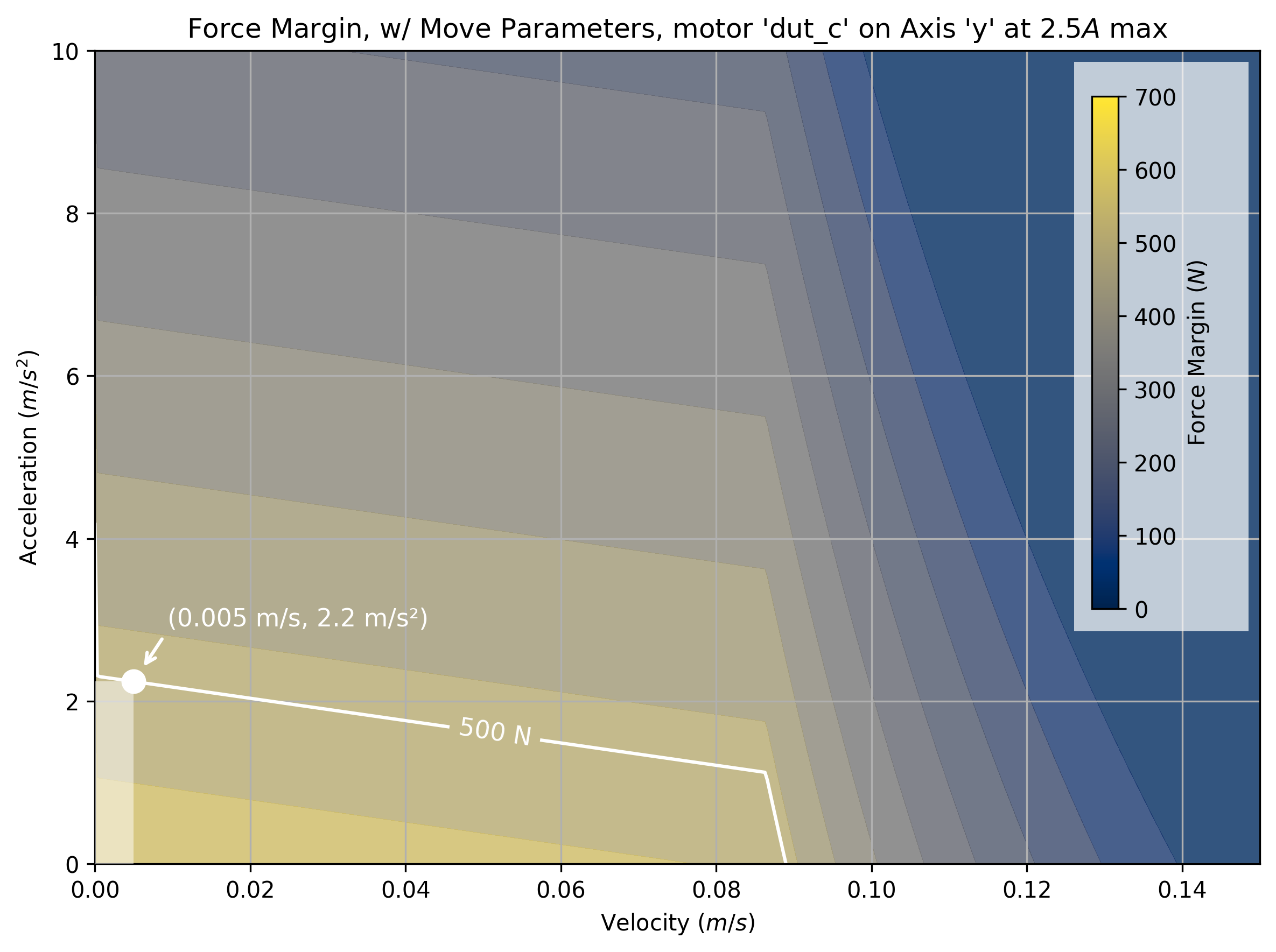
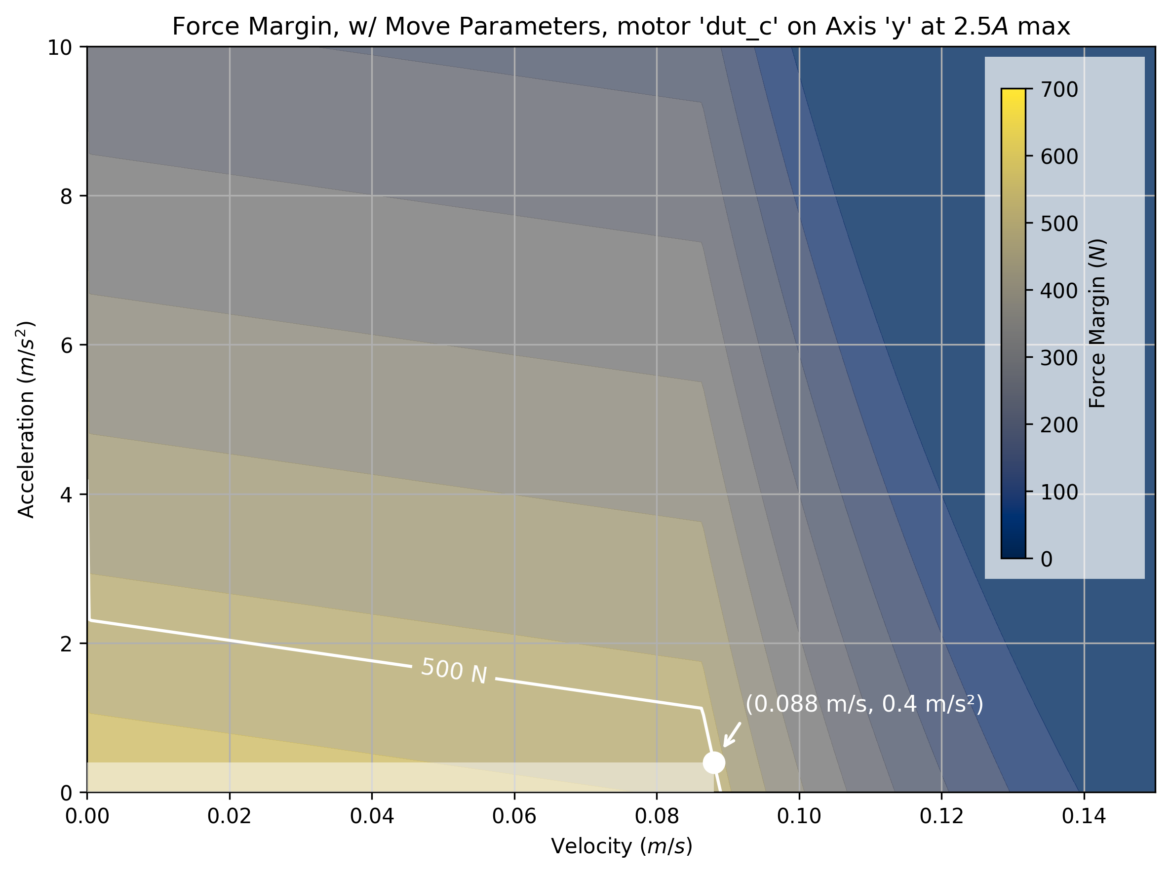
CNC Machines need to move around while providing cutting forces. To compare motor selections in this context, I developed a force margin analysis tool. Here, motor models define how much current can be generated in the motor stator as a function of the rotor speed. Using this model, and the motors’ \(k_t\) value \((A/Nm)\), we can estimate the amount of torque generated across these speeds. We can then combine this estimate with the kinematic model’s estimate for force required to accelerate the mass (just \(F=MA\)) and use the model’s damping terms to estiamte forces lost to friction.
The tool takes a maximum current saturation parameter, and a generates a force margin (maximum available force from the motor, less forces taken up by motion) across a grid of velocities and accelerations.

This plot can help us to select motors for our machine, and also forms the basis for the next tool, which can help us select operating parameters.
7.3.2 Selecting Motion Control Parameters using Models
Using force bandwidth plots (above), we can select (max accel, max velocity) parameter for our motion controller such that we guarantee a force bandwidth overhead in Newtons.
This is for use in a trapezoidal motion controller, which cannot use the entirety of the motor’s dynamic range (Section 5.7.1). That leaves us with a trade-off: high end speed or low-end force.
These are the core methods for selecting motors and motion parameters using models. I show how I used these methods together for our milling machine in Section 7.5.2.
7.4 Toolpath Inspection Tools
7.4.1 Visualizing Real Chipload
In this thesis I have discussed the idea of constrained optimization at length. Machines are limited by the physics of their motion systems and those are coupled into process physics. In particular I mentioned a hidden optimization in Section 1.2.4.1, where the velocity of a path plan is modified in real-time by machine controllers in order to avoid violating actuator and kinematic constraints.
Because our real-time controller is a software module, we can easily run path plans virtually to render the results of this optimization for machine operators before they run a job. In practice this just means that we run the machine controller in a configuration where it is disconnected from hardware, which is done using a change in the Pipes graph that runs the system. The motion controller’s outputs can then be rendered in 3D along particular points in the path, or as histograms that show statistics across the entire path.
In the case of this CNC machine, I use a trapezoid-based motion controller for acceleration planning (see Section 5.2.1). It’s outputs include the time-series basis spline that is normally sent to motors (and it’s velocity, acceleration and jerk states), as well as an output of the current segment’s target velocity (as specified in the path plan), as well as the type of motion segment (a G0 “Rapid” (traverse) move, or a G1 “cutting” move).
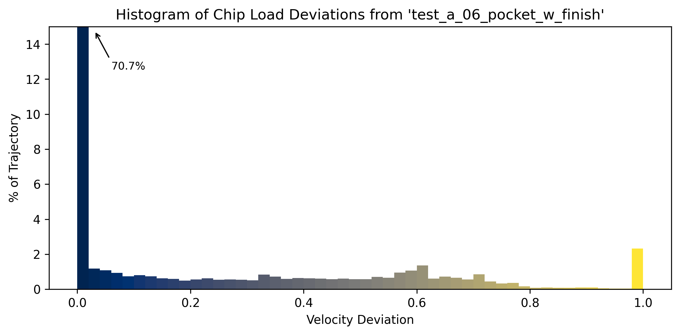
To render these outputs, I use the same 3D Plotting software as in Section 6.11.2. I measure deviation of the trajectory’s actual feedrate from the target feedrates, normalizing it into the range \(0.0-1.0\) where \(0.0\) indicates no deviation from the target feedrate, and \(1.0\) indicates a complete stop.
\[ V_{dev} = (V_{targ} - V_{norm}) / V_{targ} \]
3D Plots allow careful inspection of toolpath components. For a broader look at the toolpath’s overall deviation from target rates, we can also produce histograms of this data.
I use this tool as part of a comparison between the pocket and adaptive toolpath in 7.5.4.
7.4.2 Cutting Force Estimates
It is possible also to make cutting force estimates using a combination of real-time data from the machine and motion controller and our motor and kinematic models.
While the machine operates, we collect time-series data from the motors on their positions, velocities, accelerations, and their measurements for motor current. A complete table of data collected from motors during operation is available in Table 5.2. With the motor model (Section 5.3.1), we know that current is directly related to motor torque. Our machine’s drive ratios relate these torques to linear forces per axes, meaning that we can make a time-series of force vectors that were exerted into the machine’s axes during operation.
Much of that force is used only to accelerate and move the machine around. However, our kinematic models can estimate those currents for any velocity and acceleration. That means that we can develop a time series that combines our total force (a motor-model based measurement) with motive force (a kinematic-model based estimate) to calculate residual forces.
\[ \begin{aligned} F_{meas} = I_m \cdot k_t \\ F_{est} = F_f(vel, accel) \\ F_{cut} = F_{meas} - F_{est} \\ \end{aligned} \]
In this step, I additionally filter both force estimates before combining them using a second order butterworth filter (Butterworth et al. 1930) with \(\omega=20.0Hz\) passed through scipy’s filtfilt function (to eliminate changes in the measurement’s phase).
I use this tool as part of a comparison between the pocket and adaptive toolpath in 7.5.4.
7.5 Results and Discussion
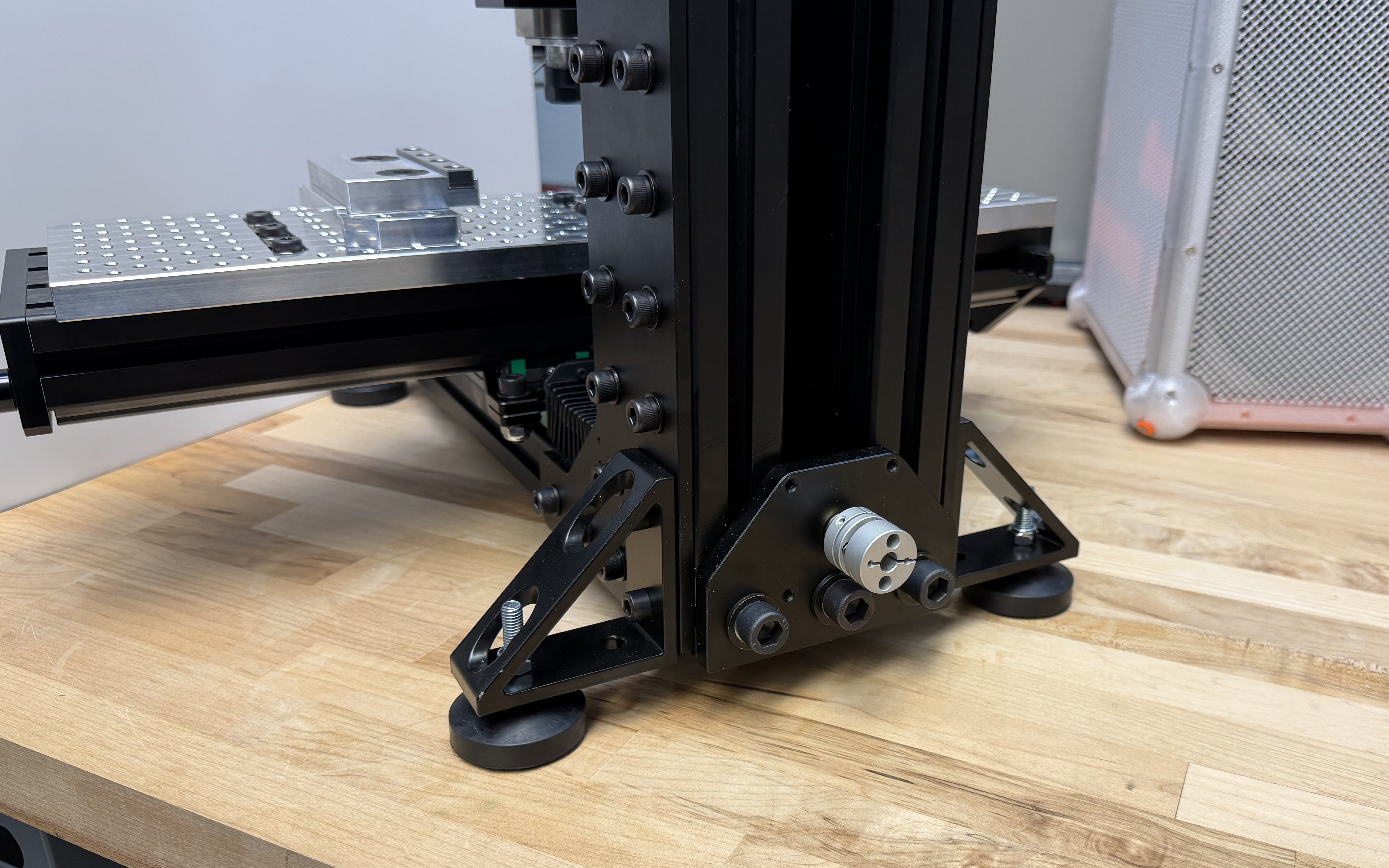
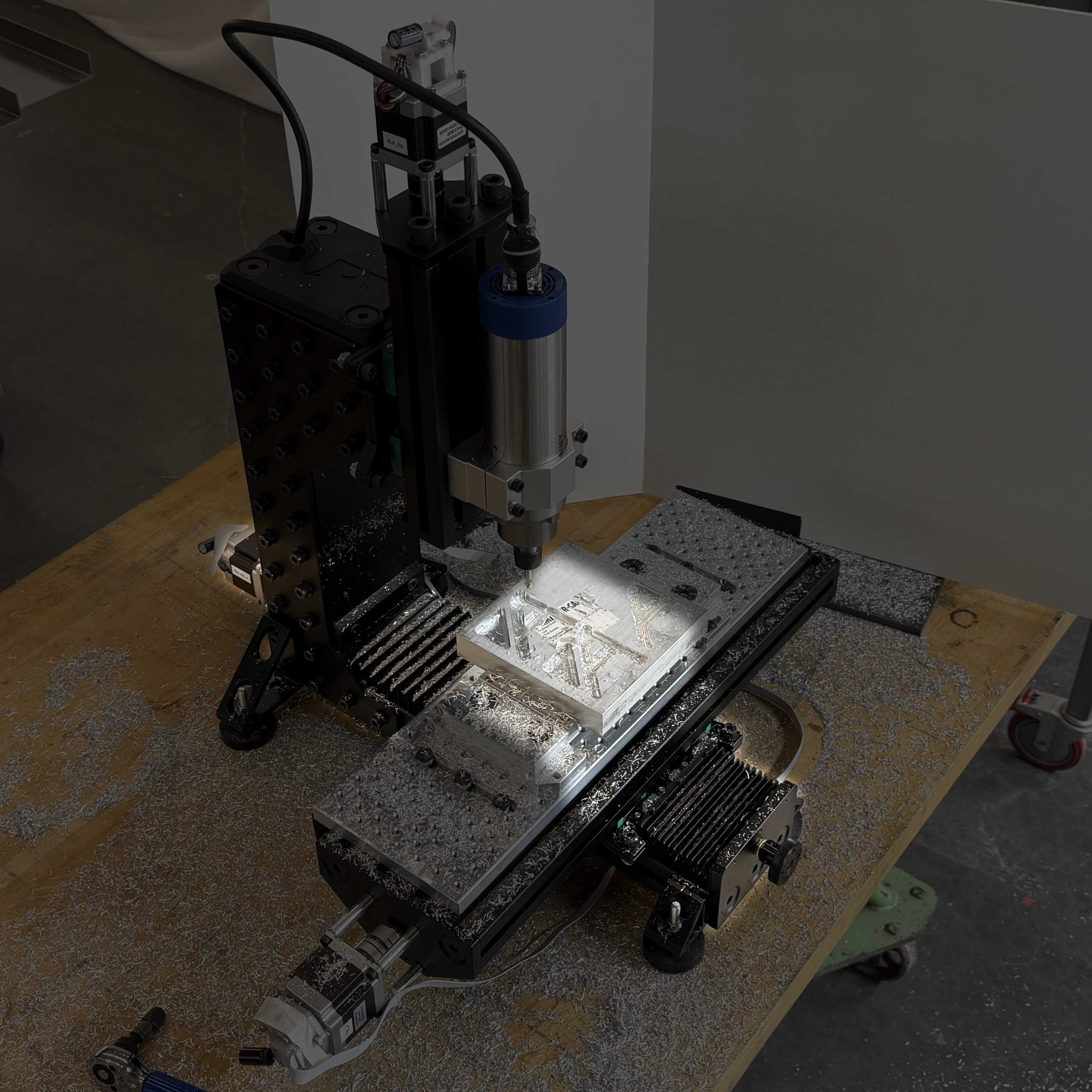
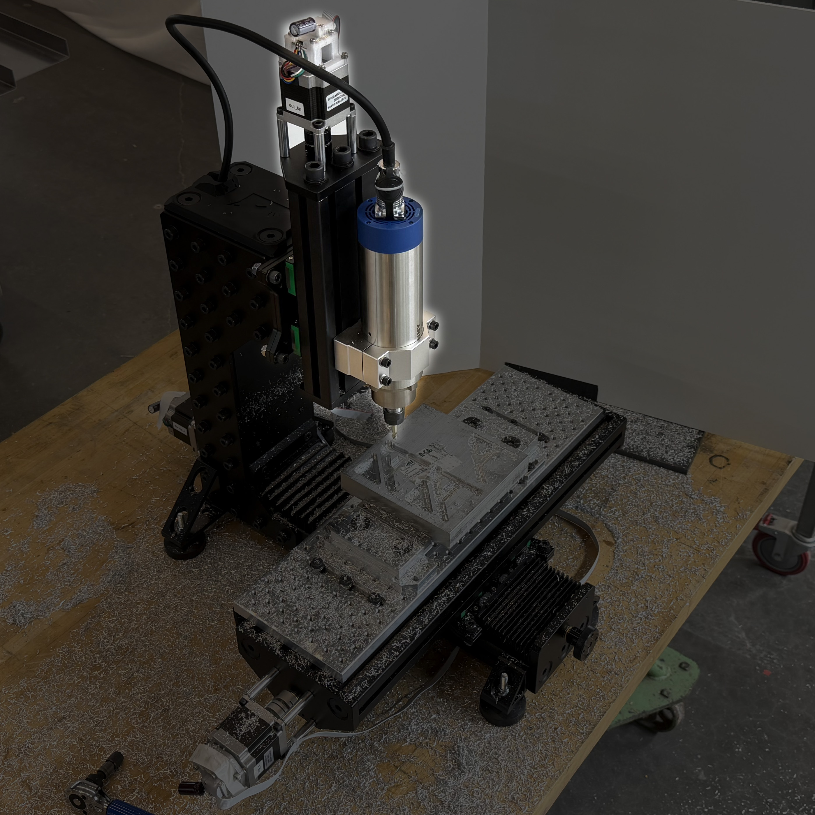
7.5.1 Hardware Developed and Tested
I used the tools and methods described in this chapter to outfit a small milling machine. The machine was assembled from a Rat Rig Mill kit (2024) and a GPenny Spindle which is rated to 1.5kW (about two horsepower) and runs up to 24000 RPM (2019). The spindle has an ER16 collet and is 65mm in diameter, and is controlled by a generic VFD powered on single phase 110V.
![]()
I added a Saunder’s Machine Works fixture plate and vise (2020), and outfit the machine with my own motor controllers (from Section 5.4), picking motors using the process described below in 7.5.2. The motion system runs on a 48V switched-mode power supply, to which I added 10000uF of capacitance and two 47 Ohm bleed resistors (in series) to help linearize it.
7.5.2 Model-Based Selection of Motors and Motion Parameters for CNC
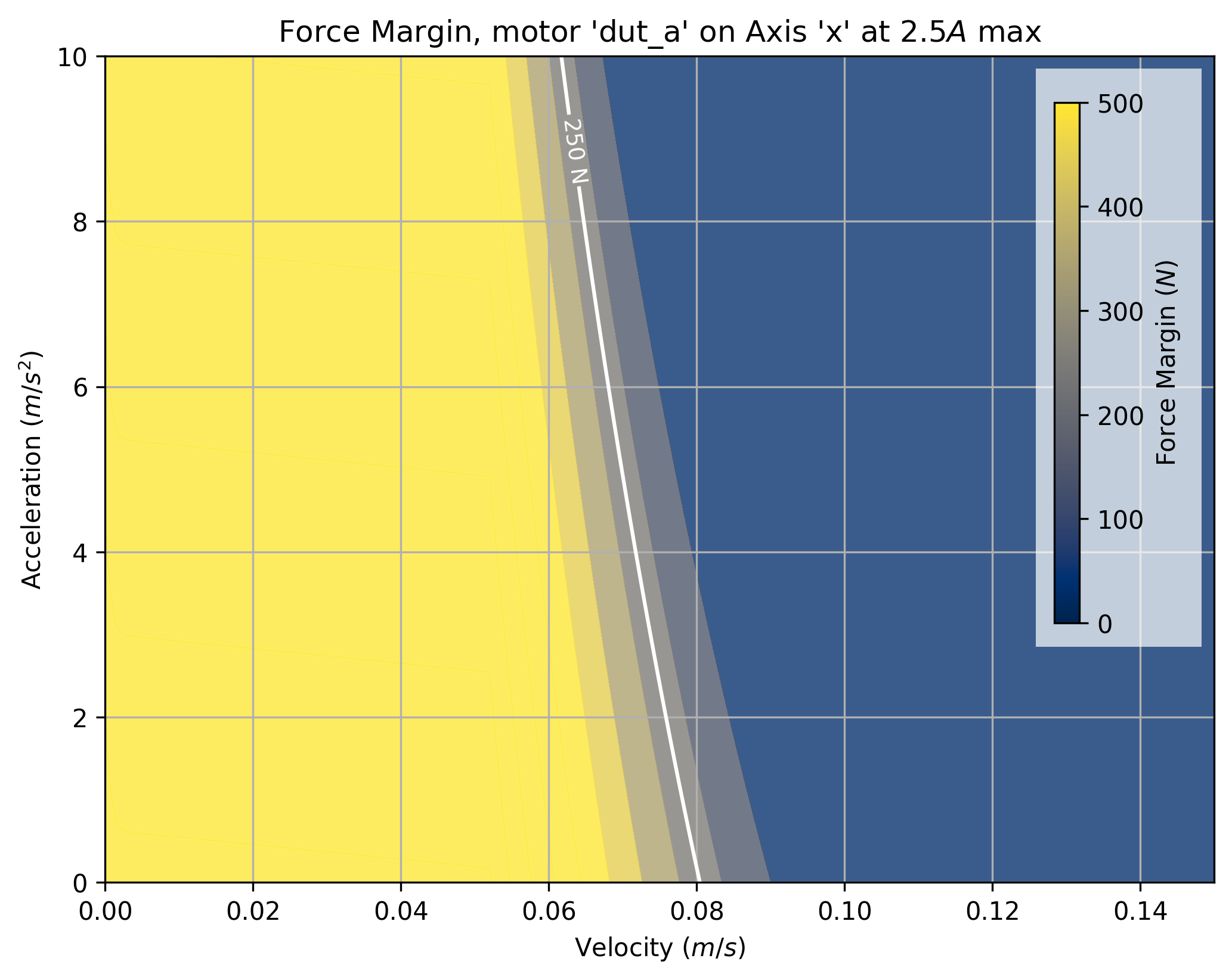
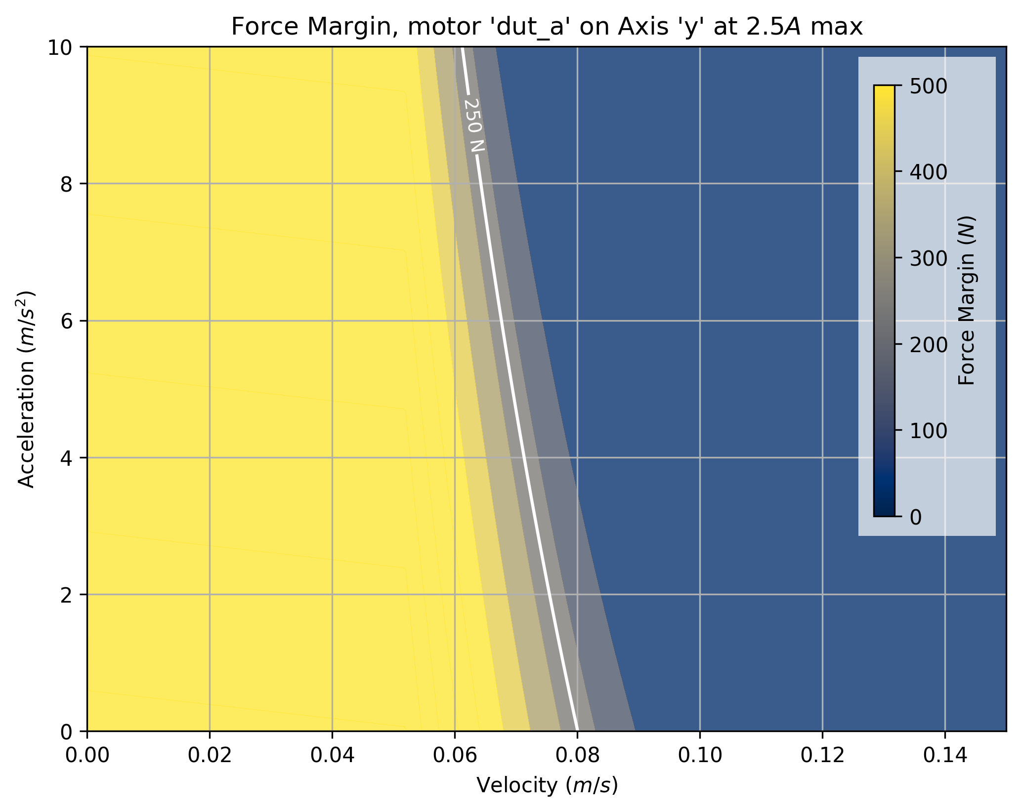
In this subsection, I explain how I used the tools developed in 7.3.1 (alongside heuristics!) to select motors for use in the CNC Mill above. I was able to assess the hypothetical performance of each axis using each motor (a total of twelve combinations) to select the motors that would provide the desired force bandwidth in the range of speeds that I expected to drive the machine.
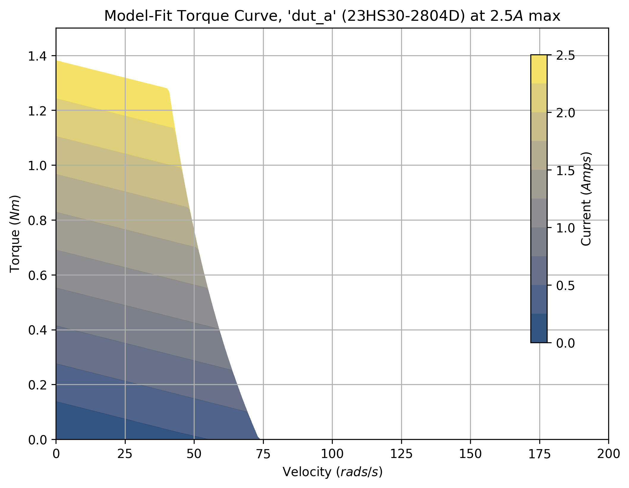
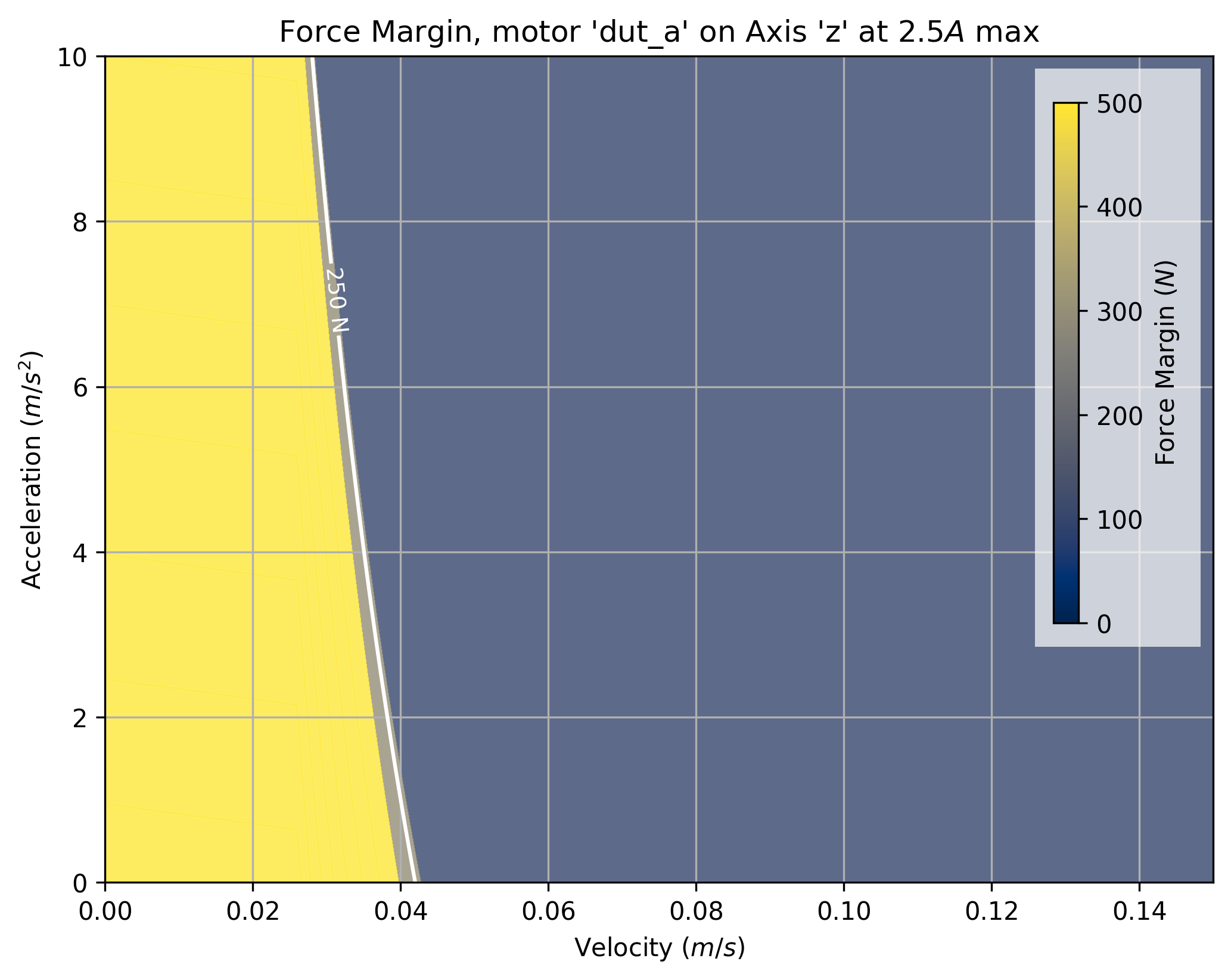
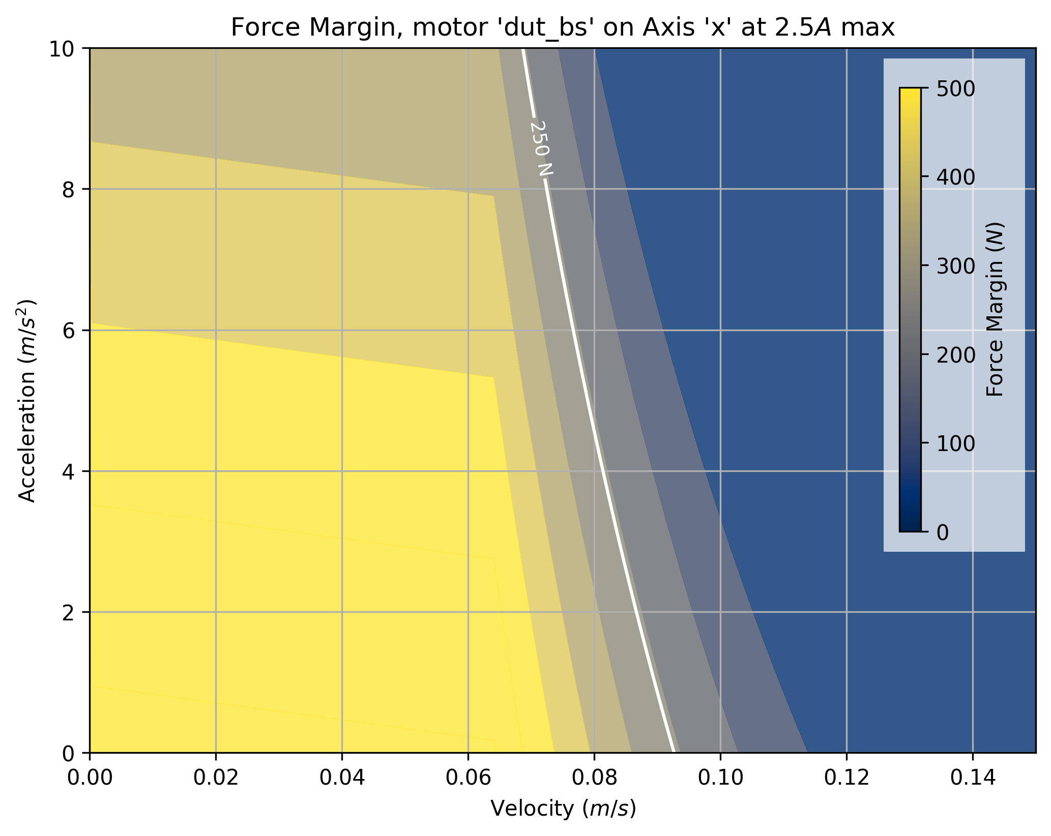
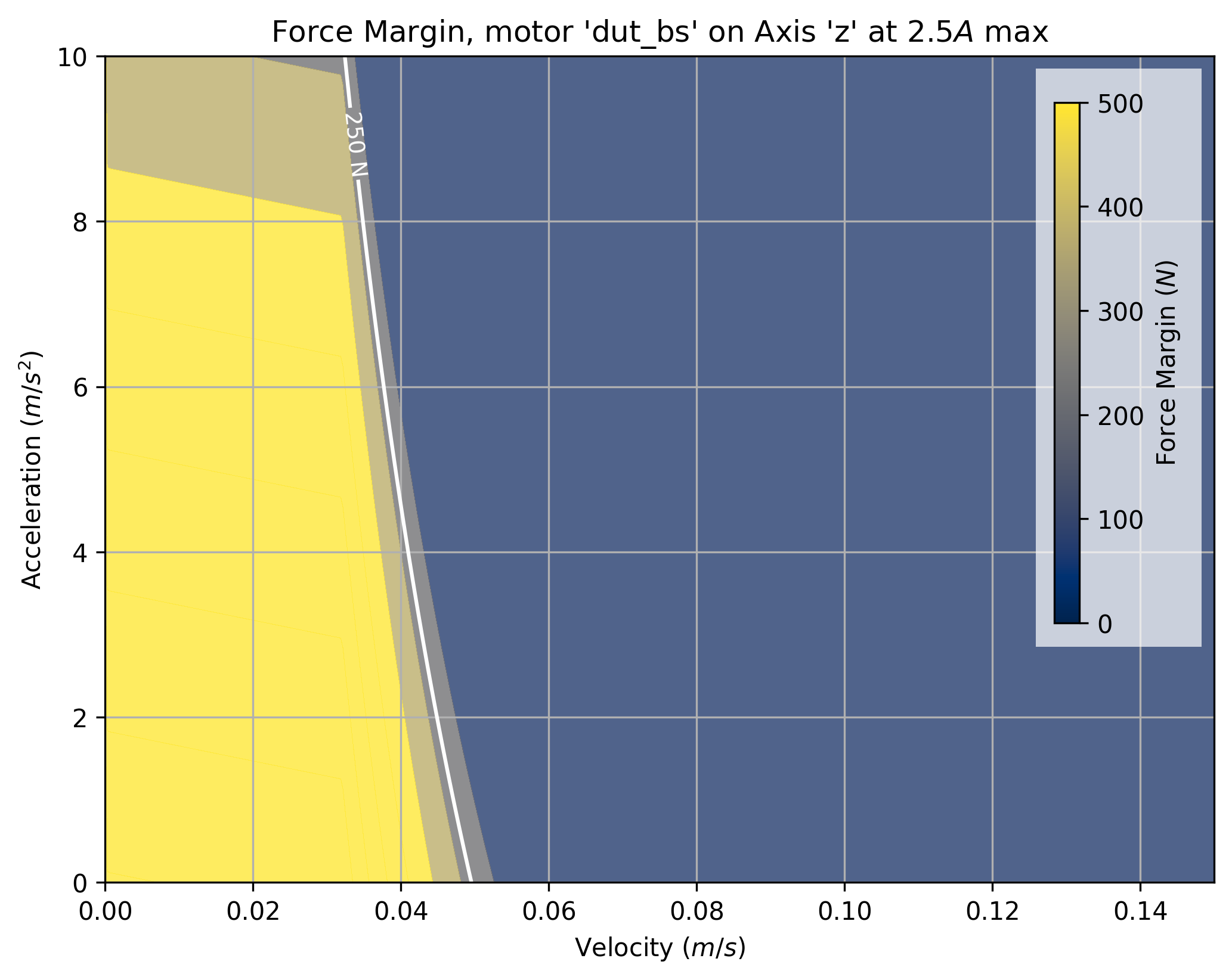
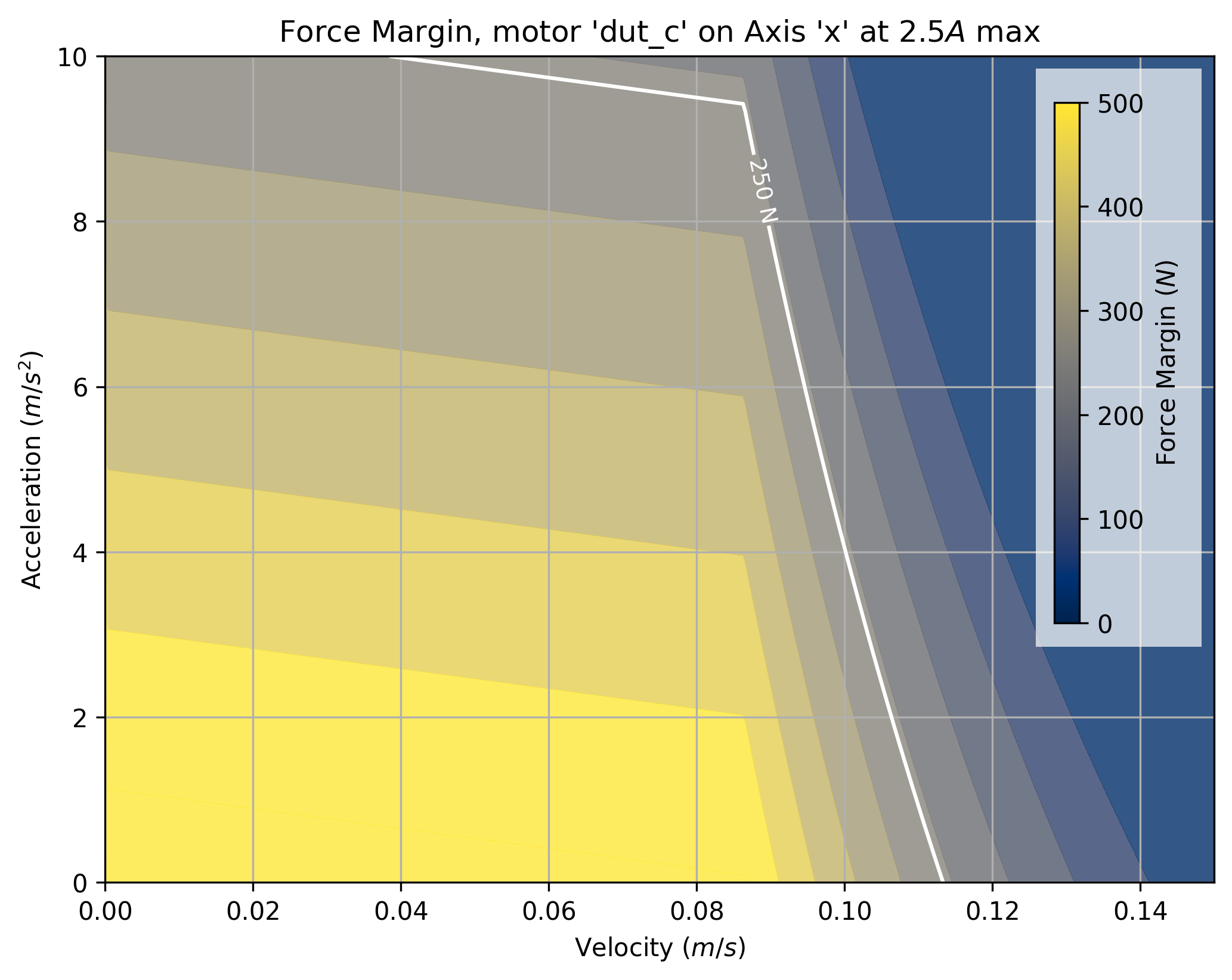
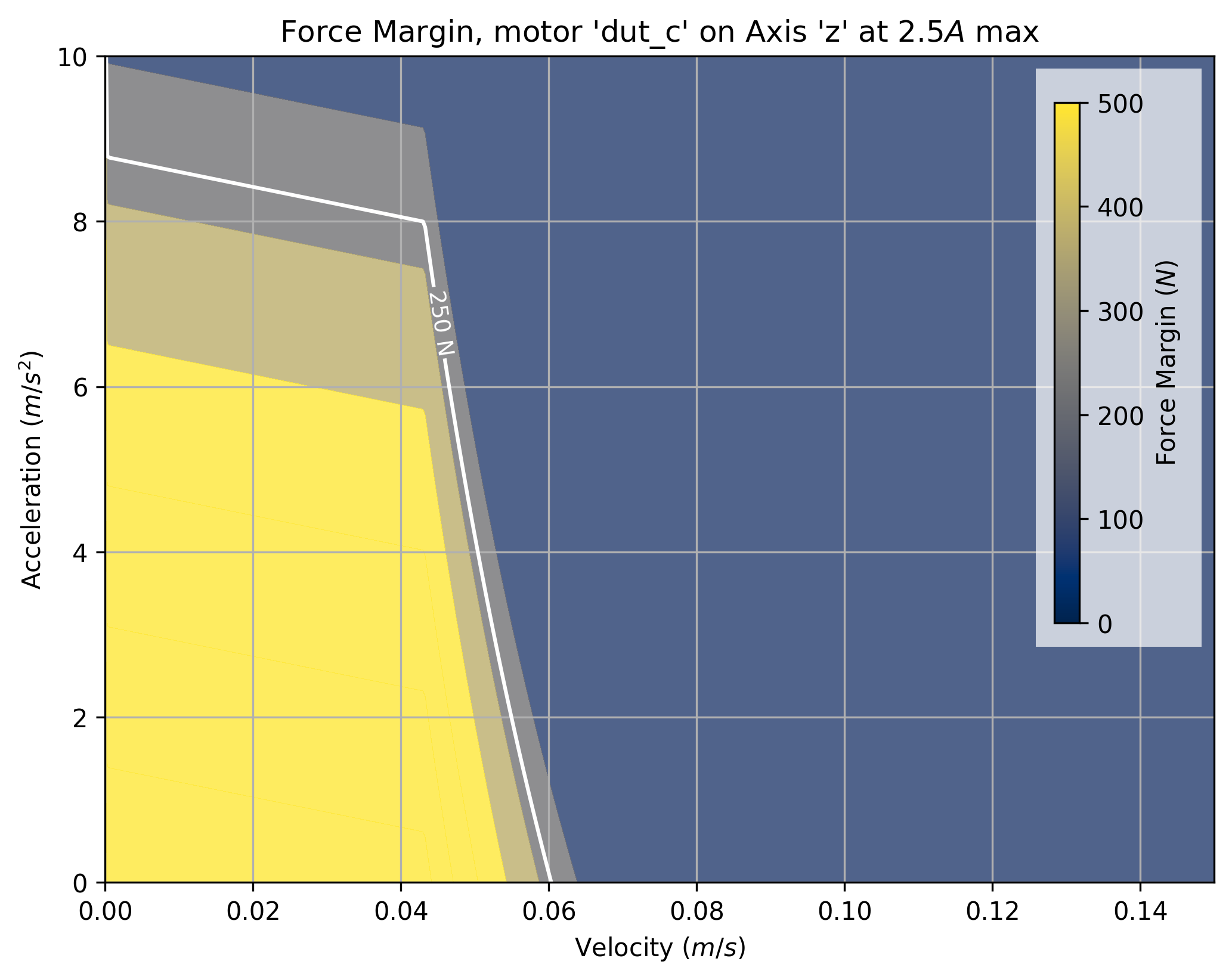
I selected four candidate motors from our stock bins at the CBA. Each is a NEMA23 size (a faceplate dimension standard, and a requirement of our machine’s frame), but have varying electrical properties and lengths. I used the method from 5.3.1 to generate an encoder calibration and model for each (this takes about 10 minutes per motor). The resulting torque curves are plotted below, and parameters are tabulated in 7.1, where I include values also for the motor that Rat Rig specifies for the CNC kit.
![]()
![]()
![]()
![]()
| Name | dut_a | dut_bs | dut_c | dut_bp | MFG |
|---|---|---|---|---|---|
| Size | NEMA23x76 | NEMA23x56 | NEMA23x56 | NEMA23x56 | NEMA23x86 |
| \(\tau_0\) | \(1.85\) | \(1.26\) | \(1.20\) | \(1.26\) | \(2.45\) |
| \(A_{max}\) | \(2.80\) | \(2.12\) | \(2.80\) | \(4.24\) | \(3.00\) |
| \(R (ohms)\) | \(1.13\) | \(1.50\) | \(0.95\) | \(0.38\) | \(1.2\) |
| \(L (mH)\) | \(4.80\) | \(4.40\) | \(3.00\) | \(1.10\) | \(4.0\) |
| \(J_{rot} (g \cdot cm^2)\) | \(480\) | \(300\) | \(300\) | \(300\) | \(670\) |
| \(k_t\) | \(0.553\) | \(0.371\) | \(0.323\) | \(0.193\) | n/a |
| \(k_e\) | \(0.572\) | \(0.399\) | \(0.331\) | \(0.245\) | n/a |
| \(k_d\) | \(0.0025\) | \(0.00064\) | \(0.00093\) | \(0.0010\) | n/a |
| \(v_{max} (rads/s)\) | \(75\) | \(104\) | \(125\) | \(165\) | n/a |
To generate kinematic models, I used the methods described in 5.3.2. In brief, this involved mounting one motor on each axis (I made a preliminary selection of dut_c for this, as it sits in the middle of the range of available performance), and having the motor follow a chirp signal using a set of preliminary PID gains. Parameters from those model fits are below, showing the machine’s relatively large damping terms \((k_{d,offset}, k_d)\) that are a result of it’s leadscrew transmissions.
| Axis | X | Y | Z |
|---|---|---|---|
| Drive Ratio \((mm/rad)\) | \(1.27324\) | \(1.27324\) | \(0.63662\) |
| Moving Mass \((kg)\) | \(9.932\) | \(10.818\) | \(4.392\) |
| J motor \((kg \cdot m^2)\) | \(0.00003\) | \(0.00003\) | \(0.00003\) |
| J coupler \((kg \cdot m^2)\) | \(0.000002873\) | \(0.000002873\) | \(0.000003180\) |
| J leadscrew \((kg \cdot m^2)\) | \(0.000001419\) | \(0.000001469\) | \(0.000000706\) |
| \(k_{d, offset} (N)\) | \(58.95\) | \(60.27\) | \(202.6\) |
| \(k_d (N/(m/s))\) | \(375.0\) | \(439.6\) | \(1602.4\) |
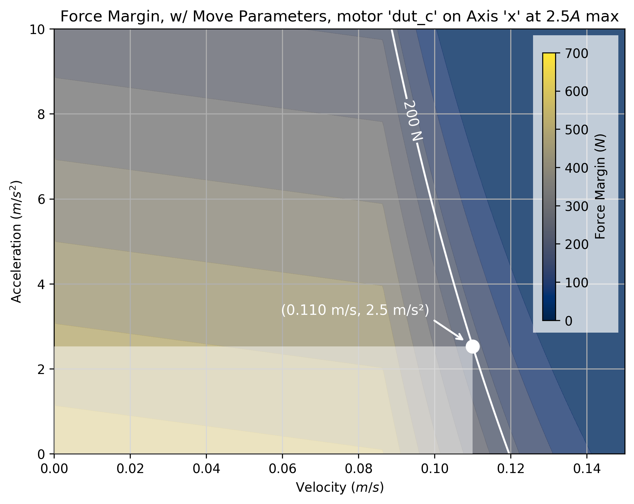
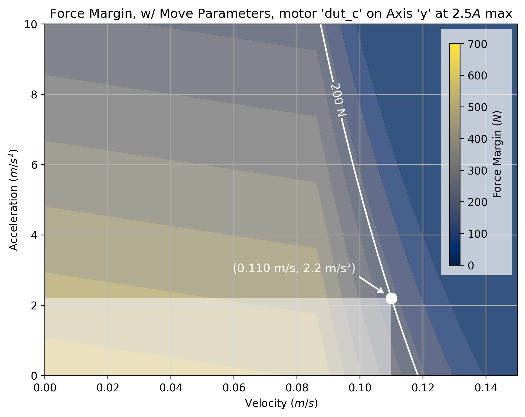
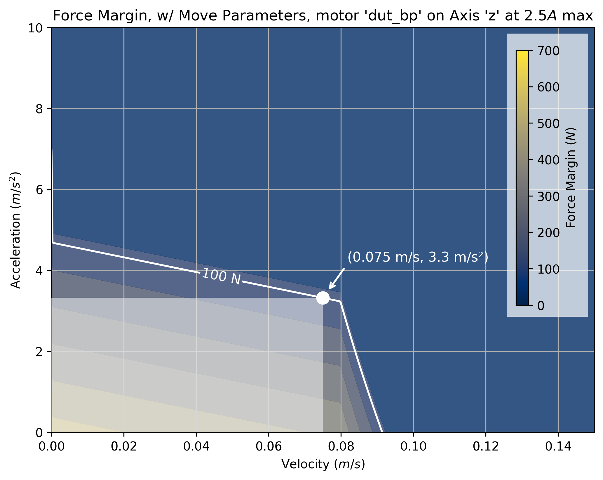
I then combined motor models and kinematic models to produce a force margin plot for the expected performance of each. For each axis, I generated four hypothetical combinations (one with each motor). I show each of those combinations in 7.11.
\(axes \otimes motors\)
![]()
![]()

![]()
![]()
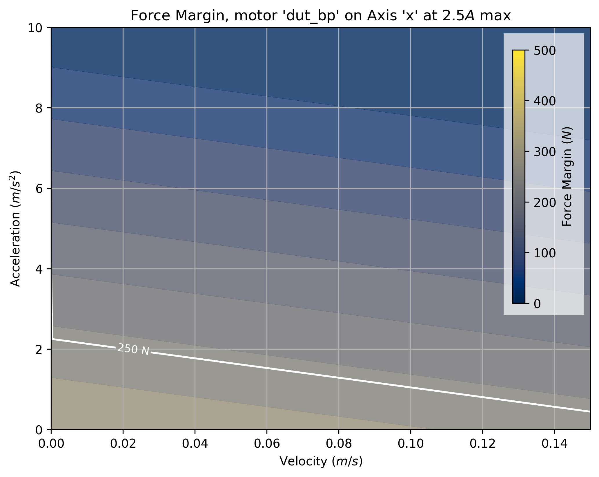
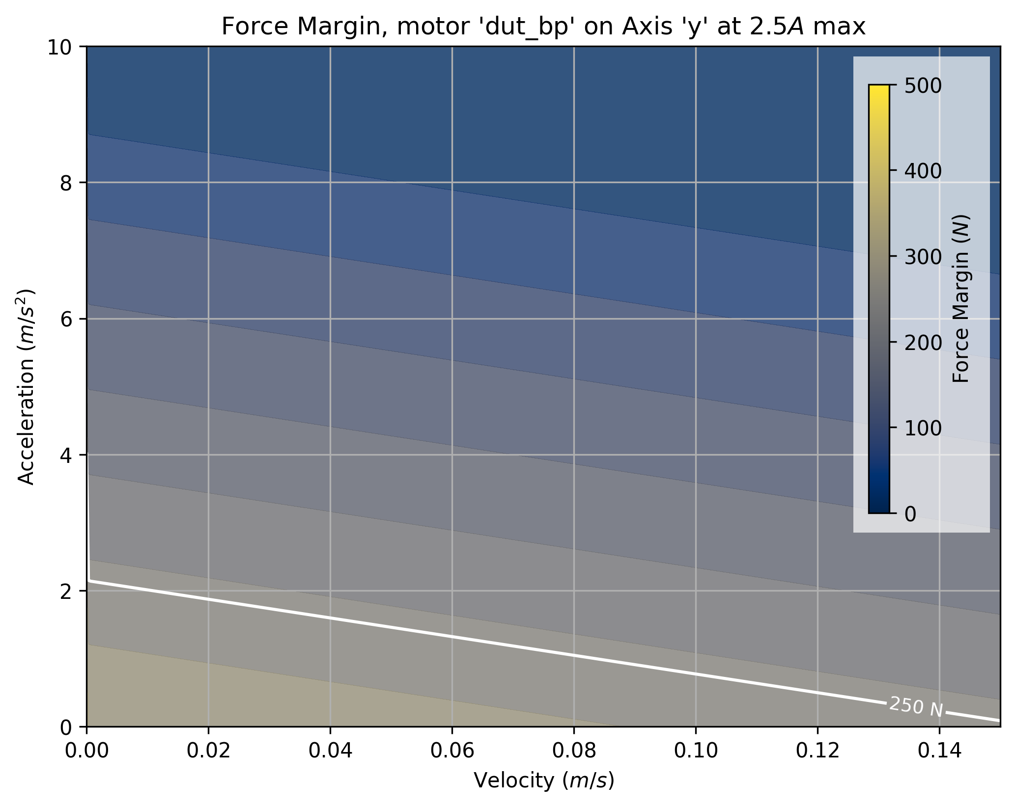
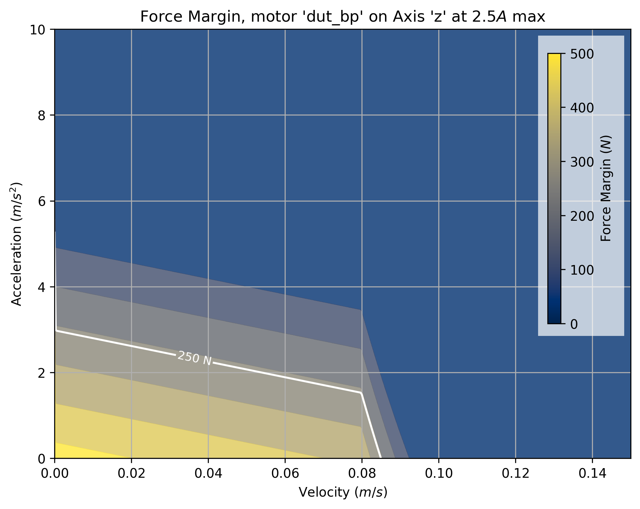
- Using these models, we can see that the z axis’ increased drive ratio (it uses a 4mm lead screw, whereas x and y use an 8mm lead screw) leads to - unsurprisingly - smaller achievable feedrates overall. It also has punishing damping terms.
- Heuristically, we know that maintaining high feedrates is important for machining with a low-ridigity machine, to keep overall removal rates up without exerting large forces.
- We can turn this heuristic into a force margin, supposing we only plan to exert 200N (about 20kgf) on the machine during operation in \(x\) and \(y\), and half of that in \(z\) where cutting forces are lower (we tend to plunge more gently).
- Then we can select towards higher feedrates, so long as we maintain an (heuristically) high acceleration. Since machining involves many retracts in the \(z\) axis, we favor acceleration over maximum speed on this axis.
- Discussion has to include: this is a demonstration of the use of these tools; my own expertise is the main deciding factor here. The point is not that these tools supplant or replace expert knowledge, it is that they can help us to make more precise decisions, and build understanding of our machines…
| Axis | X | Y | Z |
|---|---|---|---|
| Motor Selection (ours) | dut_c | dut_c | dut_bp |
| Motor Selection (model) | 23HS22-2804D | 23HS22-2804D | 23HS22-3008DP |
| Motor Selection (mfg) | LDO-57STH86 | LDO-57STH86 | LDO-57STH86 |
| Force Margin (ours) \((N)\) | \(100\) | \(200\) | \(200\) |
| Force Margin (mfg) \((N)\) | n/a | n/a | n/a |
| Max Velocity (ours) \((mm/s)\) | \(110\) | \(110\) | \(75\) |
| Max Velocity (mfg) \((mm/s)\) | \(50\) | \(50\) | \(25\) |
| Max Acceleration (ours) \((mm/s^2)\) | \(2500\) | \(2200\) | \(3300\) |
| Max Acceleration (mfg) \((mm/s^2)\) | \(300\) | \(300\) | \(200\) |
In the table above, I show the final motion parameters and force margins selected using this process. I also include parameters from the CNC machine kit manufacturer’s recommended setup.
In summary, this process is preferrable over the state of the art because it enables us to rapidly compare more possible design outcomes using real data from our hardware, rather than estimates. The simple metric here is that we were able to use four motor models and three axis models (each of which is fit in tens of minutes) to evaluate twelve combinations of each. Done manually (swapping each motor onto each axis) may take a day or longer. In addition, the models we use allow us to simulate operation across a wider range of parameters than those where we test them, and our controller allows us to virtually test the entire machine in a number of configurations.
This process also led to the selection of dramatically improved motion parameters over the manufacturer’s recommended settings: 2x (xy axes) and 3x (z axis) increase in top speeds and 8x (xy axes) and 16x (z axis) increases in acceleration. The manufacturer selected motors have much higher rated holding torque over my selections, but a torque curve for their motor seems to be unavailable, meaning that they may have selected motors based on holding torque alone without analyzing performance at high speeds. Their selections surely also encode many of their heuristics, so we may simply differ in that regard. They also deploy open-loop steppers, where loss of a single step can be extremely troublesome, whereas our closed-loop motors allow us to push closer to the machine’s limits without worrying about occasional hiccups. That is to say, their margins to machine performance are probably much larger.
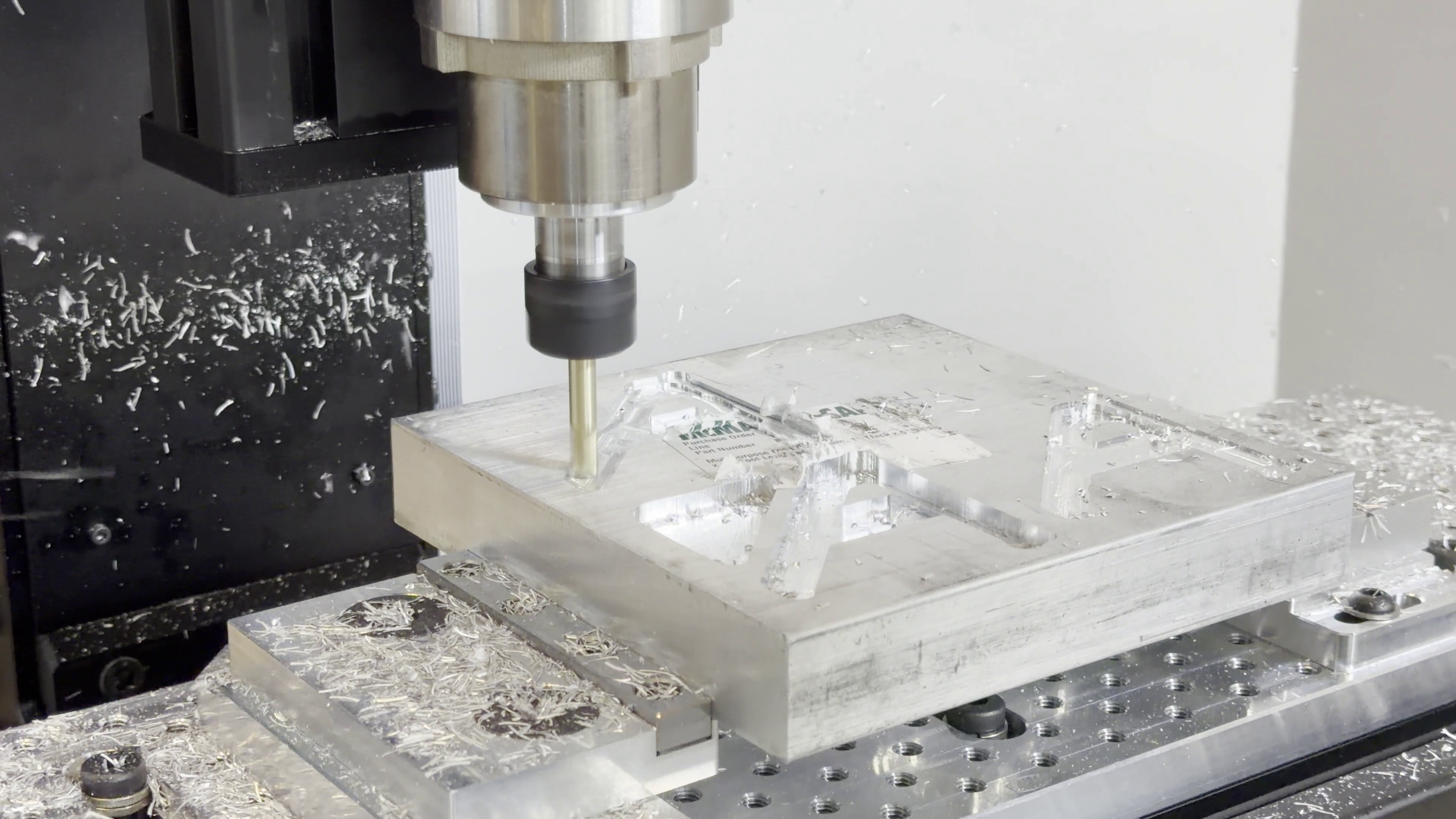
7.5.3 Machining with Models
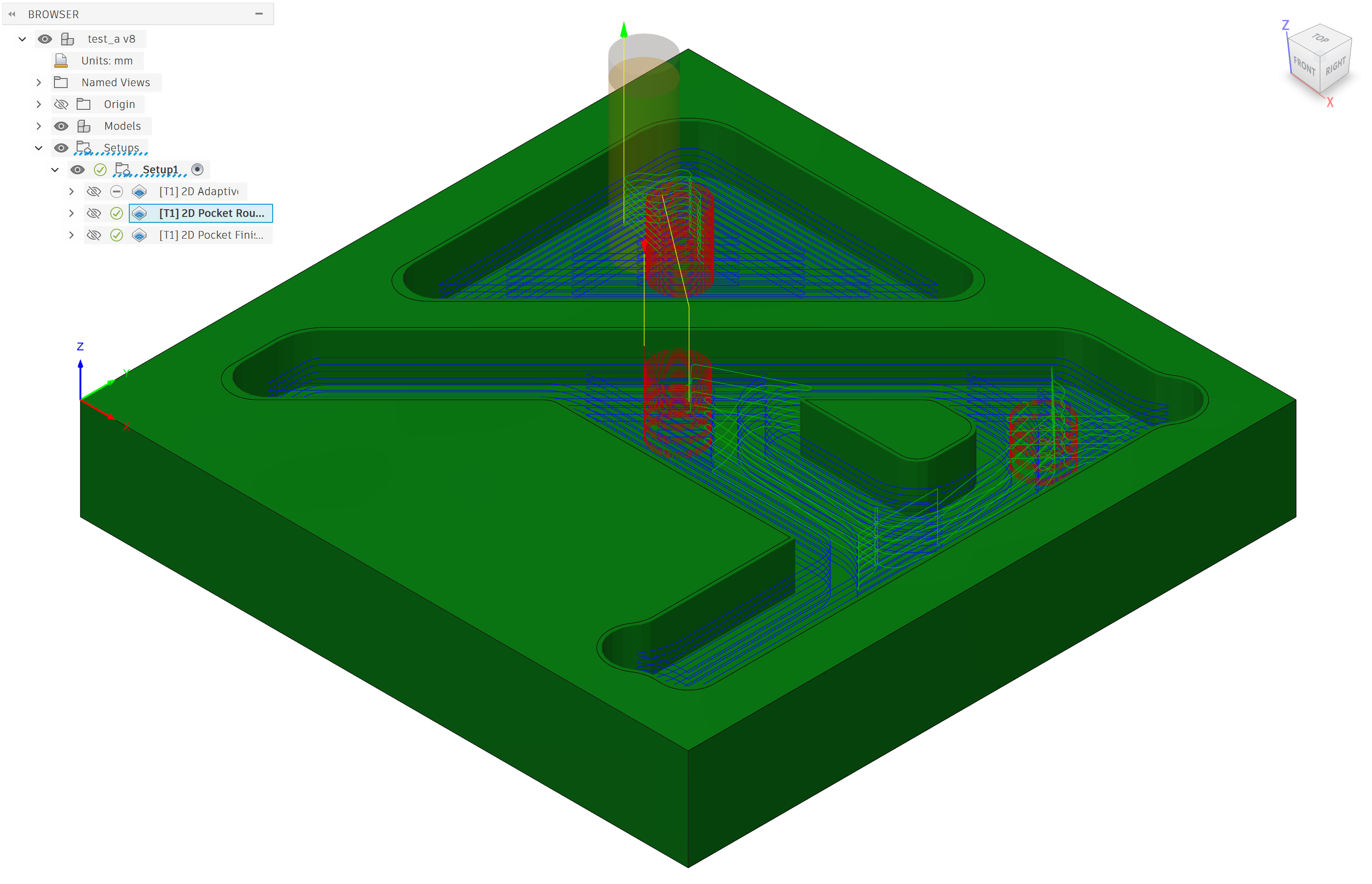
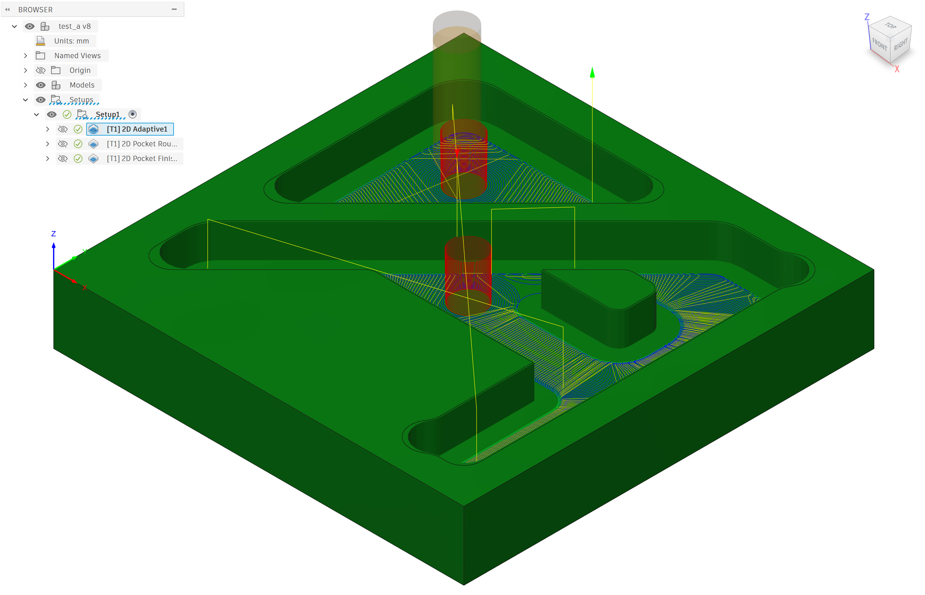
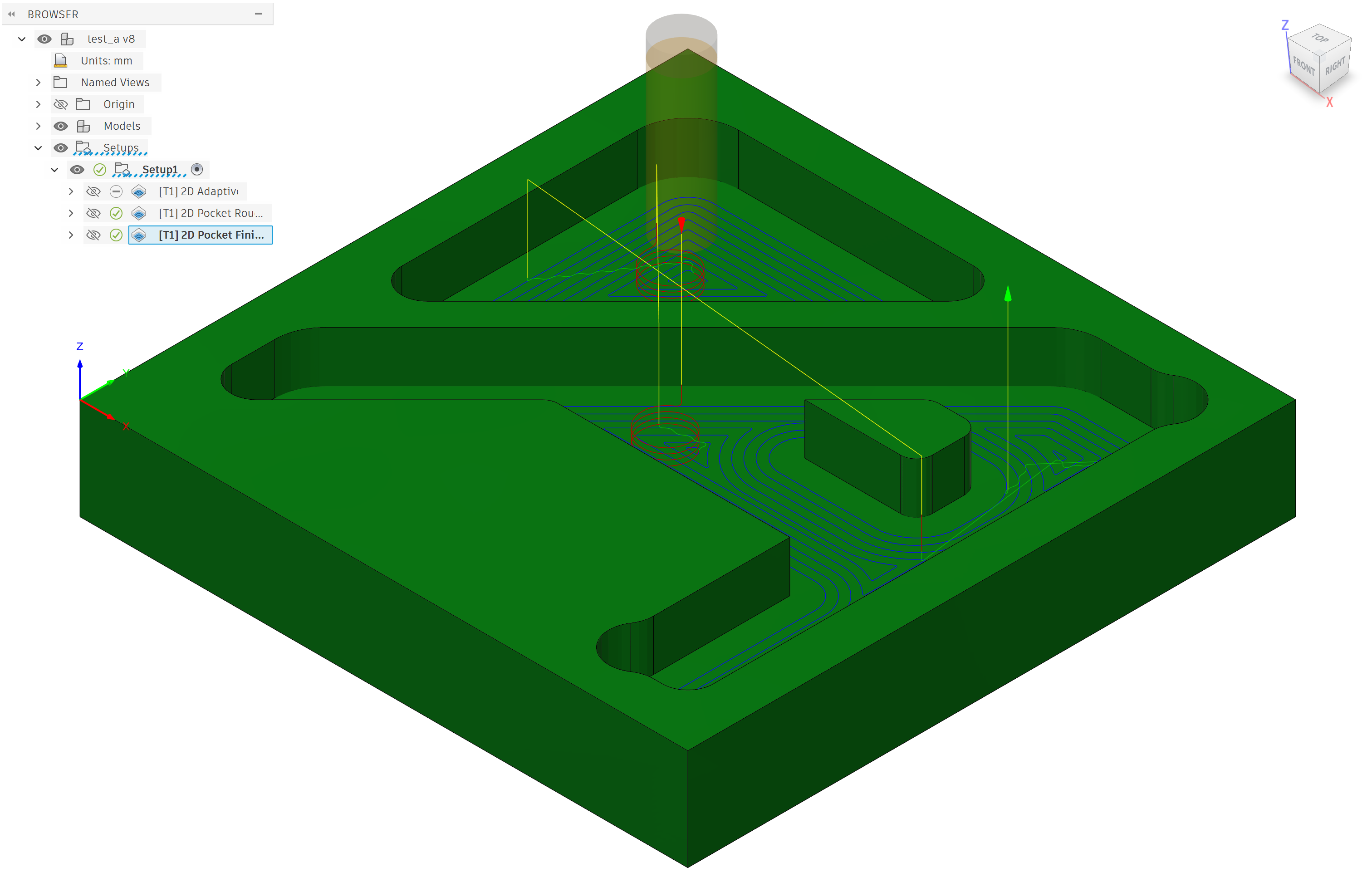
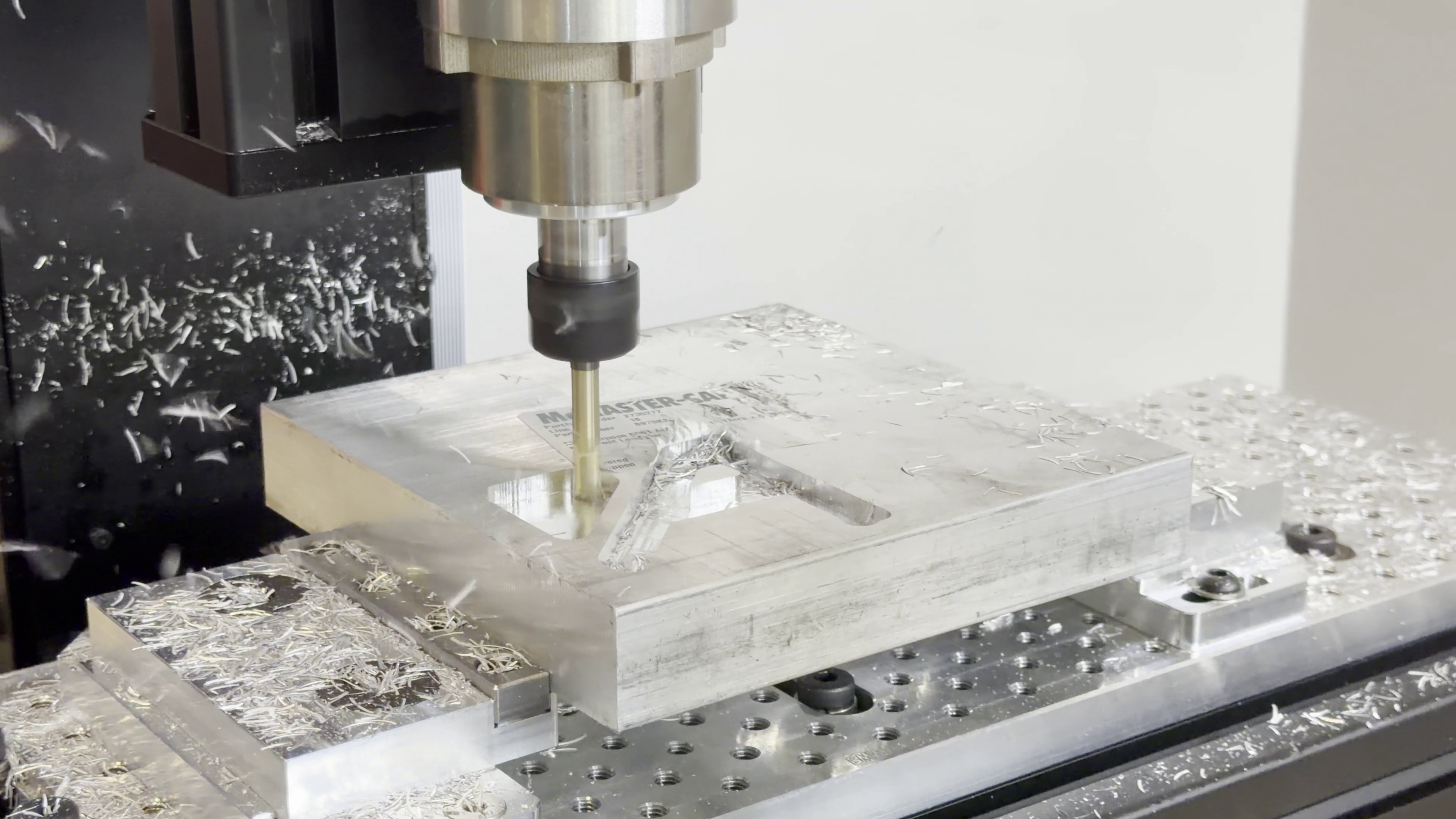
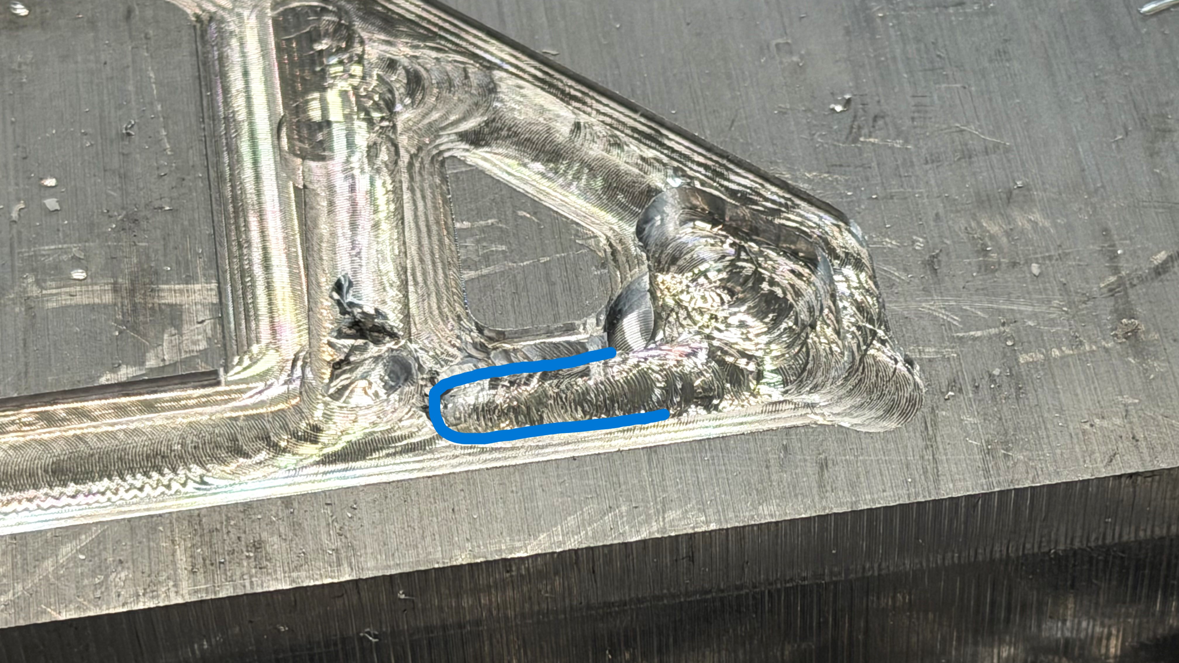
I modeled a small test piece, test_a, with two bosses at 1/4” depth each, to mill out of aluminum. The part is small, but I tried to include some common geometric features: small islands, both rounded and sharp corners, and dogbones, which are relieved sharp corners of roughly the same diameter as the cutting tool (bottom left and far right of each figure below).
I generated three toolpaths for this part using Autodesk Fusion version 2701.1.18. I selected a three-flute helical endmill at 1/4” diameter, which I thought would approximately saturate the spindle power during high speed machining. The toolpaths generated (see Figure 7.12 and paramters in Table 7.4 below) include a conventional pocket where voids are milled using concentrically increasing paths that are offset from the pocket edge, and an adaptive clearing toolpath, which is a “high speed machining” strategy that clears pockets using a series of smaller arcs. The third toolpath is another pocket, setup as a finishing pass: it clears a small amount of material that is intentionally left over during higher speed, higher load operations (to produce a smoother finish).
All three toolpaths are configured to generate the same chip load, using the spindle’s maximum RPM and relatively high linear feed rates. The chip load value was selected heuristically, using mine and our shop director Dan Gilbert’s own knowledge in machining. However, the machining strategies have different cutter engagement areas (cut depth x cut width). The adaptive path strategy is developed to maintain a uniform engagement area, avoiding slotting (where the tool cuts across its full width) by generating a series of small arcs to traverse through narrow sections. The pocket toolpath does not do this, and so its engagement area is variable - again, see Table 7.4 for numerical values.
| Final Parameters Used | Value | Meaning |
|---|---|---|
| All Toolpaths | ||
| Spindle RPM | \(24000RPM\) | Spindle’s rotational speed. |
| Surface Speed | \(478m/min\) | Speed at cutting edge. |
| Cutting Feedrate | \(78mm/s\) | Translational rate. |
| Chip Load | \(0.065mm\) | Linear translation per endmill tooth appearance. |
| Ramp Angle | \(0.6^\circ\) | Helical angle for plunges. |
| Ramp Diameter | \(6mm\) | Helical diameter for plunges. |
| Pocket Toolpath | ||
| Stepover | \(2.5mm\) | Depth of cut. |
| Stepdown | \(0.75mm\) | Width of cut. |
| Cut Engagement Area | \(1.875-4.763mm^2\) | Area of cut \((w \cdot d)\) |
| Adaptive Toolpath | ||
| Stepover | \(0.5mm\) | |
| Stepdown | \(6.35mm\) | |
| Cut Engagement Area | \(3.175mm^2\) | |
| Finishing Pass | ||
| Stepover | \(0.4mm\) | |
| Stepdown | \(6.35mm\) | |
| Cut Engagement Area | \(2.54mm^2\) |
7.5.3.1 Discussion of the Model-Based Machining Experiments
In this subsection I am going to describe the process that I went through - using a few of my tools and a heavy helping of heuristics - to develop the parameters in Table 7.4 above. While it does not constitute a rigorous evaluation of the process, I think that it is useful to include to describe the types of workflows that modelling can aid. For reference, I am familiar with machining as a process but have not accumulated more than ten hours of total time programming CNC machines. Of course I developed an understanding for their physics during the course of this project, but my tacit knowledge in the domain is limited when compared to a “seasoned” machinist.
I developed these parameters primarily guided by chip load and cutter engagement heuristics. I tuned parameters first for the adaptive path, using the machine simulation (in particular, histograms of chip load deviation were most useful (7.8)) to select a feedrate where the motion systems’s acceleration limits (selected in 7.5.2) would not cause eggregious deviations from the target chip load during cornering.
I ran this machining job a total of six times, making small adjustments to feedrates and cutter engagement areas as I proceeded. I started with the adptive toolpath and initially selected a smaller spindle speed and only half of the final feedrate and cut depth in Table 7.4, to maintain the target chipload but minimize cutting forces on the machine as I had no sense of what those forces may be. The very first run stalled the spindle during the initial ramp in (the red helical moves in Figure 7.12), after which I halved the ramp angle. The second run (an adaptive path) was successful.
I then used the cut force estimation plots (Figure 7.9) to asses my use of the machine’s available force under real cutting conditions. Seeing that my initial parameters used only tens of newtons of (estimated) cut force during the heaviest sections of the operation, I doubled the feedrates, step-down, and spindle RPM. This maintains the target chip load, but increases the total cutting force. The limit at this point was the spindle RPM.
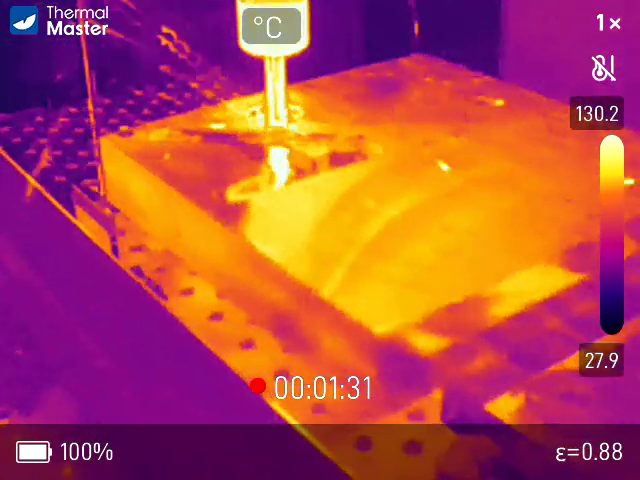
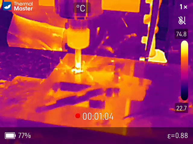
Having access to a thermal camera was an additional aid; I used this to assess whether the endmill was generating too much heat, i.e. melting metal rather than cutting it. An heuristic here is that we want to see the heat energy going into the chip rather than the part.
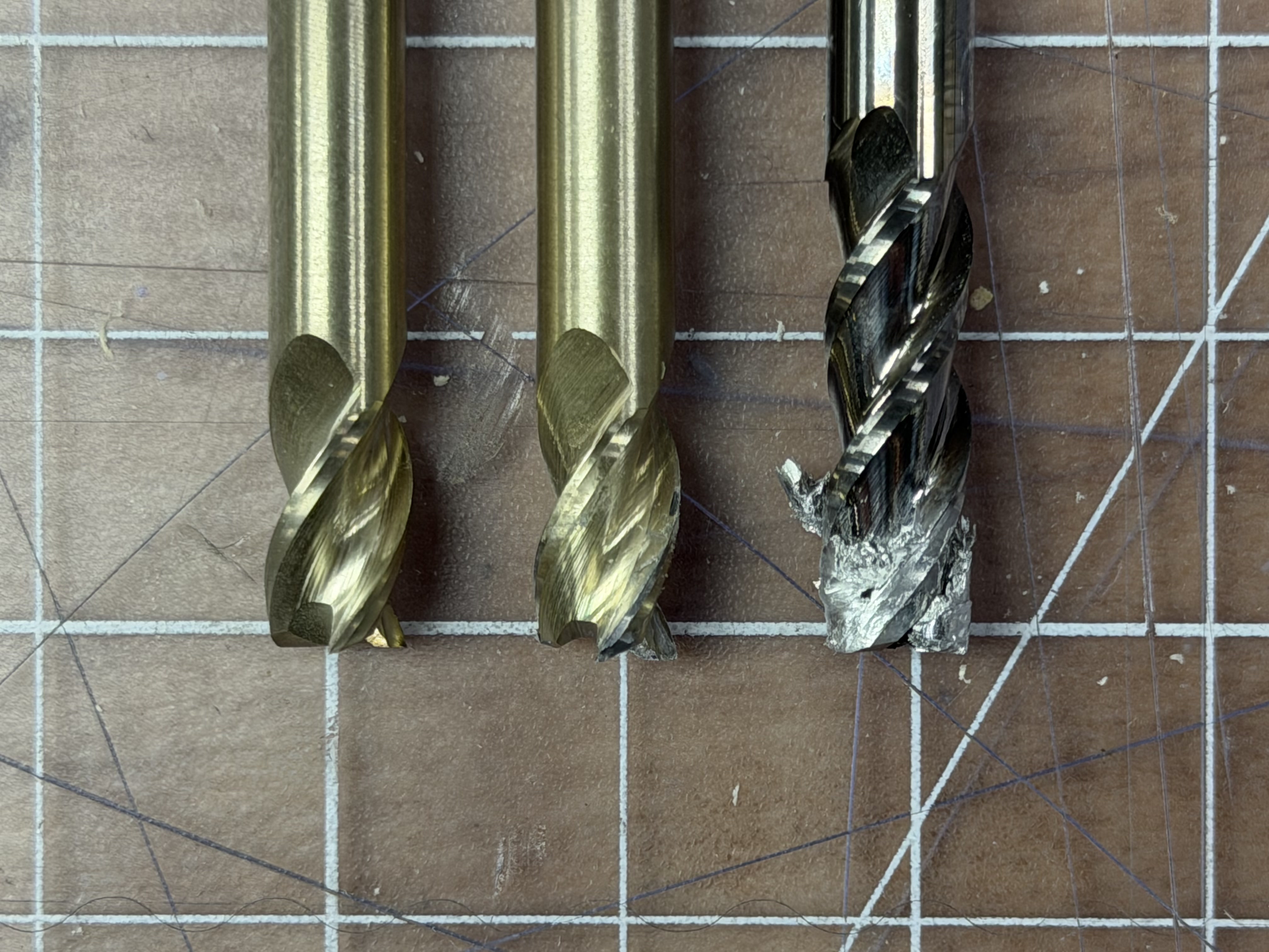
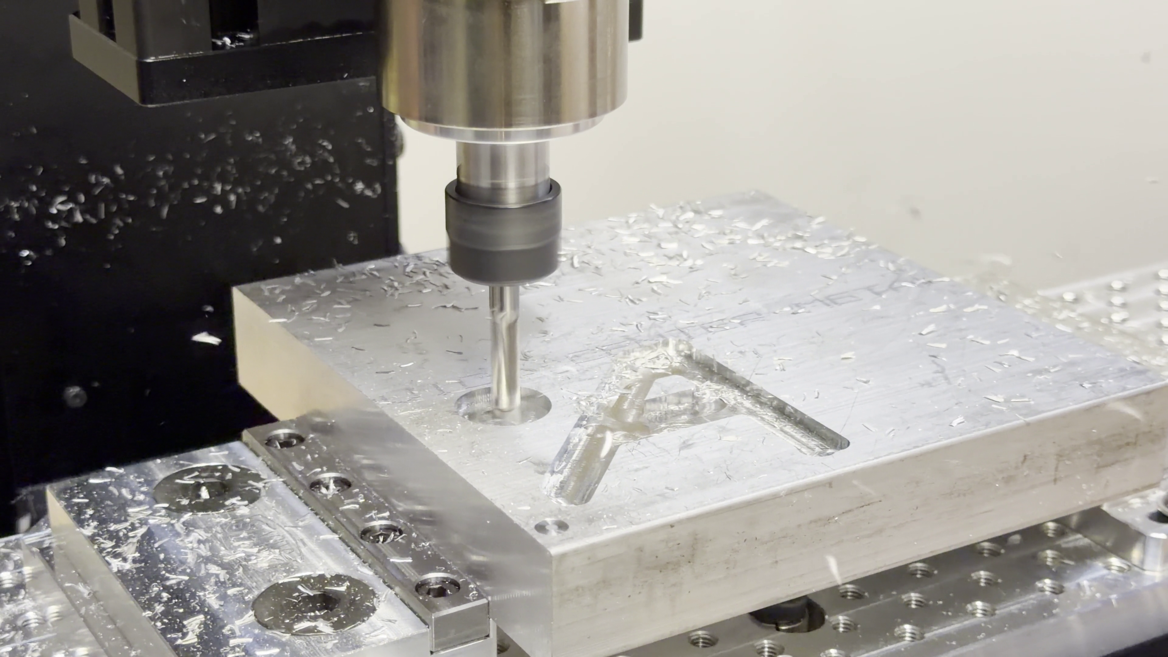
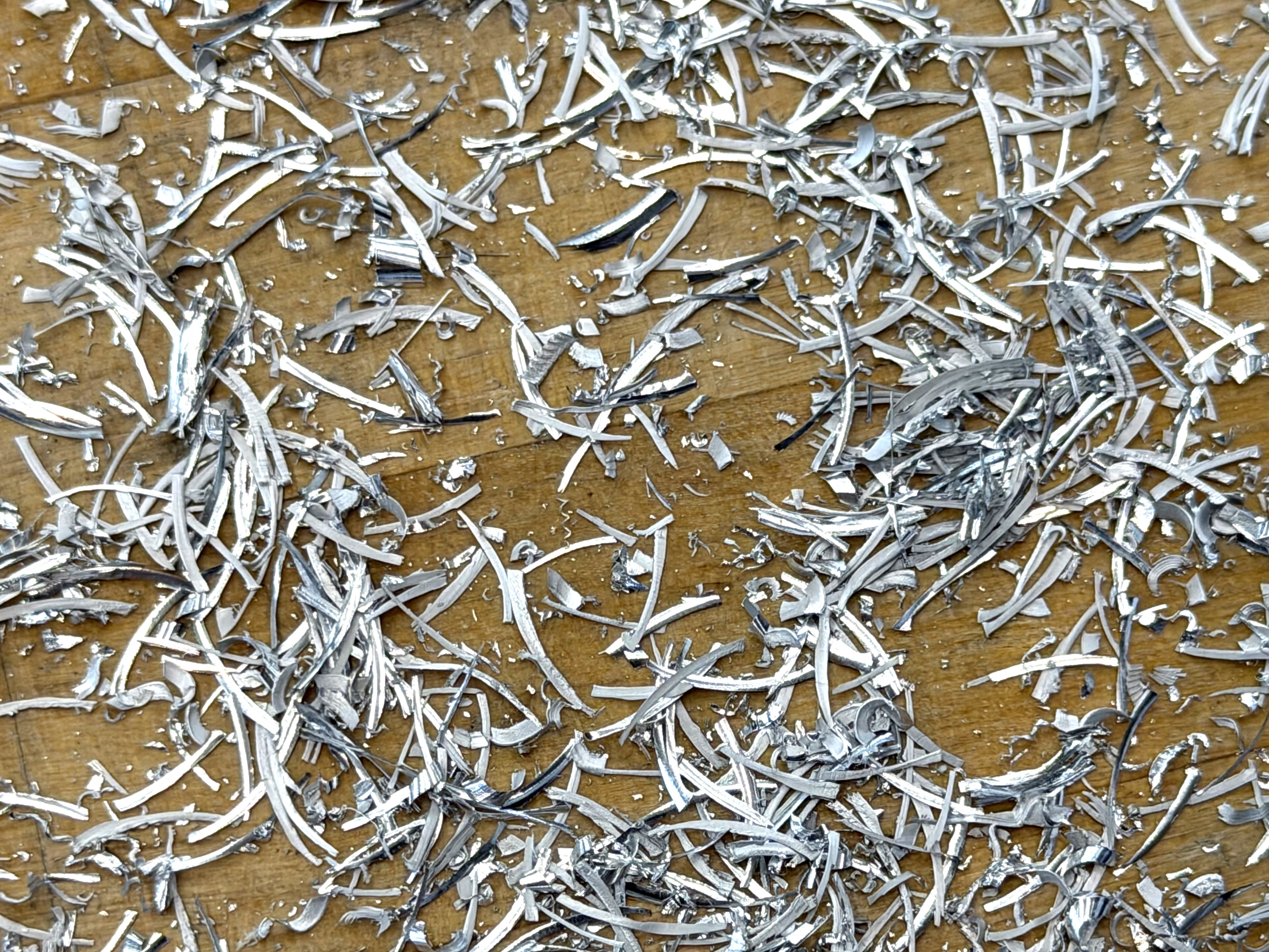
During the third test I had parameters set to the rates in the table above, except for the ramping feedrate, which I had lowered out of fear. This turned out to be the wrong intuition: the ramping rate, in combination with the higher spindle RPM, decreased the chip load such that the ramp failed again, melting the material rather than cutting it. The sacrificial endmill for this run is at right in Figure 7.2. I picked up on this for two reasons: (1) the endmill had obviously welded itself to the part and (2) the chips that were emerging at this point were much smaller than those that were thrown out of the part during the last successful cuts.
For the final test of the adaptive path, I increased the ramp feedrate to match the other paths in the toolpath. Ramping can be difficult to figure out, since cutting edges at the bottom tip of an endmill have more variable geometry than their side edges - the center of the tool also spins at “zero” RPM which presents its own set of problems that I won’t discuss at length, but you can imagine how steep ramp angles may exacerbate those issues.
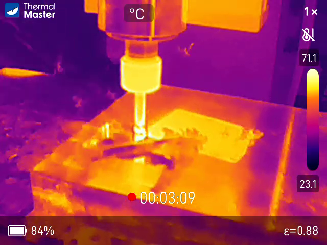
With that last adjustment, I had a good recipe for the adaptive path. One more note here is that I swapped the uncoated endmill for a similar tool with an ANF coating (Aluminum Non Ferrous). This is a proprietary PVD (Physical Vapor Deposition) coating (2020) that is designed to decrease friction and increase hardness at the tool surface, which in turn is said to reduce heat flux into the tool itself. Looking at the thermal images from Figure 7.14 and 7.16 above, (130 vs. 71 degrees at the hottest point), we can see that this holds some water.
I copied those parameters into the adaptive path, but had to find new stepover and stepdown parameters. I initially estimated that I could get away with a 2mm stepdown, to finish the part in only three depth passes. This test failed during the second step-down, stalling the spindle. I used the cutting force analysis tool to check the force exerted by the machine during that pass, and decreased the stepdown to 0.75mm, producing a total of eight depth passes. The second run of the pocket toolpath was successful.
In all, the tools I developed were useful to understand the machine’s feed and force limits, and anticipate slowdowns due to acceleration before the parts were run. These types of feedback are not available in state-of-the-art CNC workflows where motion control and process parameter selection are separated and machinists tend to rely purely on tacit knowledge and intuitions i.e. about how a machine should sound when it is operating. Here, we can add quantitative data for these analysis where it was previously unavailable.
However, I had to rely heavily on heuristics to successfully machine parts. Clearly missing from this work is a cutting force model, a spindle power model, and properly articulated heuristics or calculation of chip loads (two failures came from spindle stalls, and one from chip melting). I discuss this, and the possibility of producing real-time user (and controller) process feedback in Section 7.7.
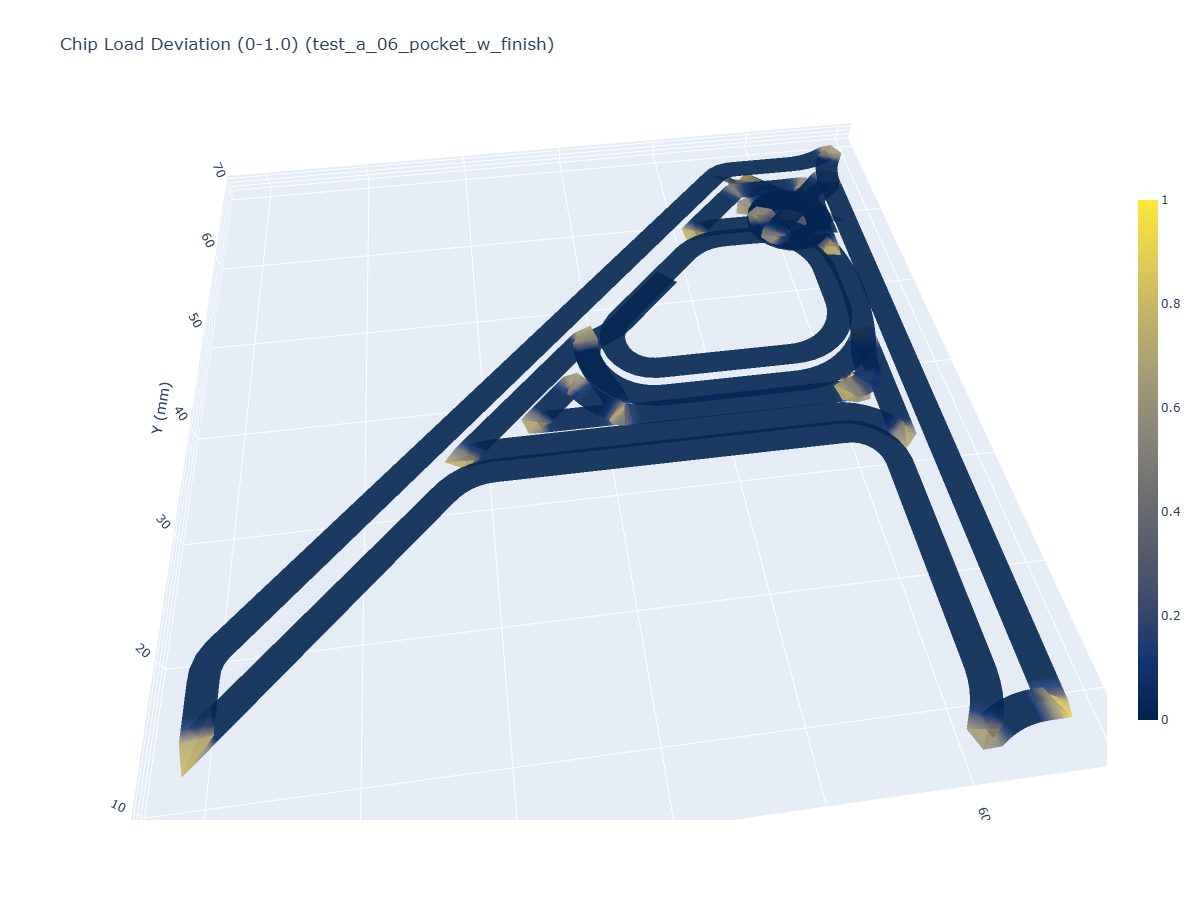
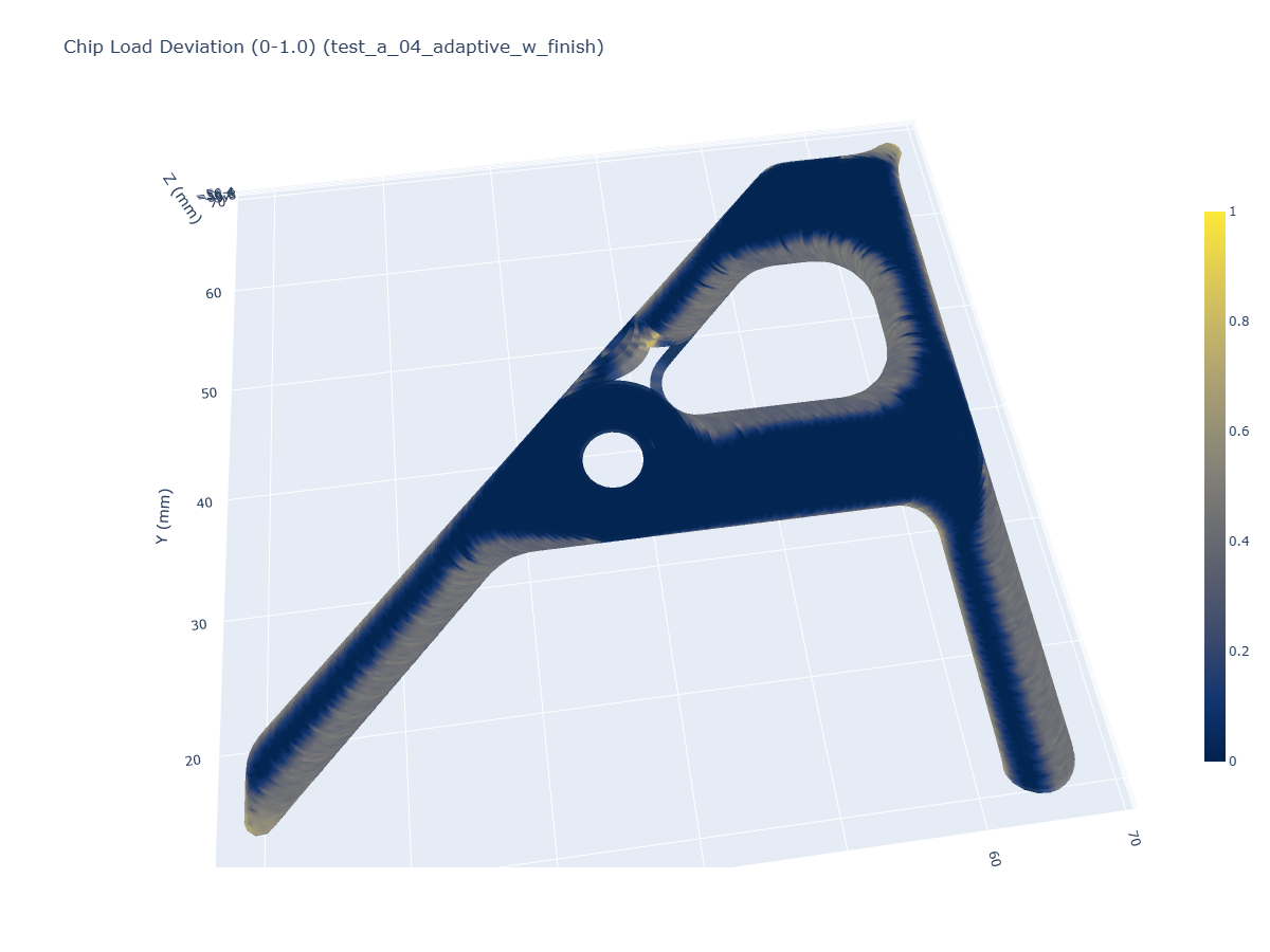
7.5.4 Chip Load Deviation and Cutting Force Estimates
“High Speed Machining” strategies like the adaptive toolpath tested here are a (relatively) new phenomenon in the CNC industry. They became possible when machine controllers became fast enough to handle the very-many small arcs and segments that they are made up of. Their operation is slightly counter-intuitive; in an adaptive path our machines spend about half of their time not cutting (circling around to the next cut), whereas traditional toolpaths engage the tool more frequently.
We can use our analysis tools to look at the differences in real machine operation across these two paths, reason about interactions between the motion controller and toolpath, and discuss limits to the current set of tools I have developed.
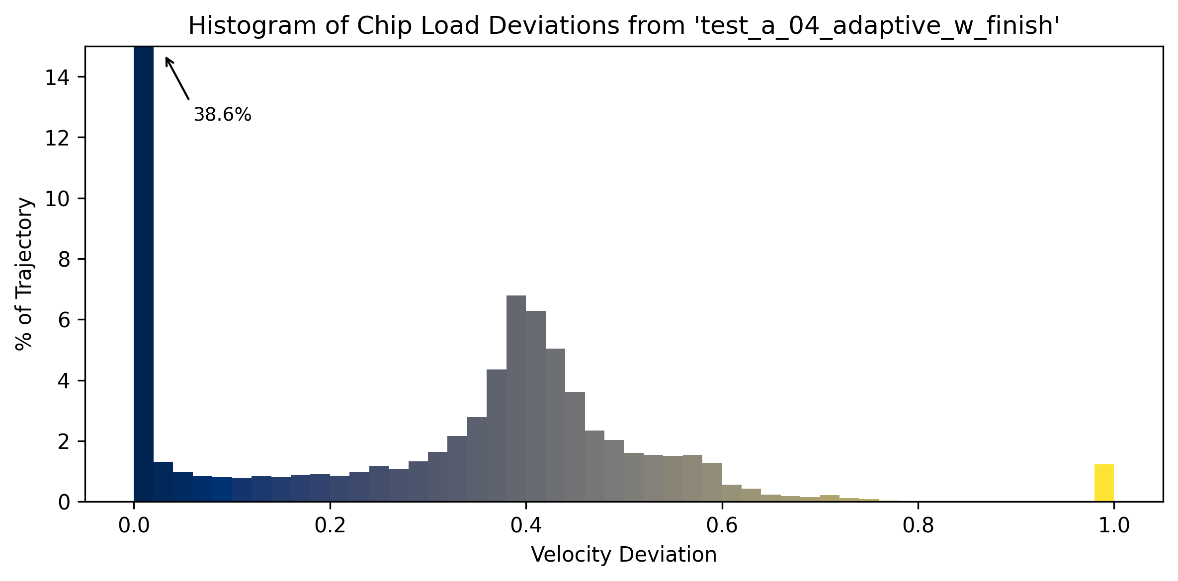
The first thing to notice is in the chip load deviation comparison above. We can see in the histograms that the pocket toolpath (left) actually deviates less overall from targets than the adaptive path (right). There is a clear concentration of deviation in the adaptive path around \(0.4,\) my estimate is that this corresponds to the cornering velocity through the chosen radius of the path’s lead-in and lead-out segments (where it turns around to start a new cut). We can see that in the 3D plot as well. These radii are also tuneable parameters in our CAM tools, and so it may be possible to use these virtual motion controllers to more intelligently pick those. In fact, ascertaining the maximum speed for a kinematic system through an arc is quite simple (so long as axes accelerations are uniform or close to it) (\(V_{max,corner} = \sqrt{A_{max}r}\)). In my tests, I used default radii from Autodesk Fusion, which are likely tuned for industrial grade machines, which obviously do not match our small CNC mill in terms of motion performance.
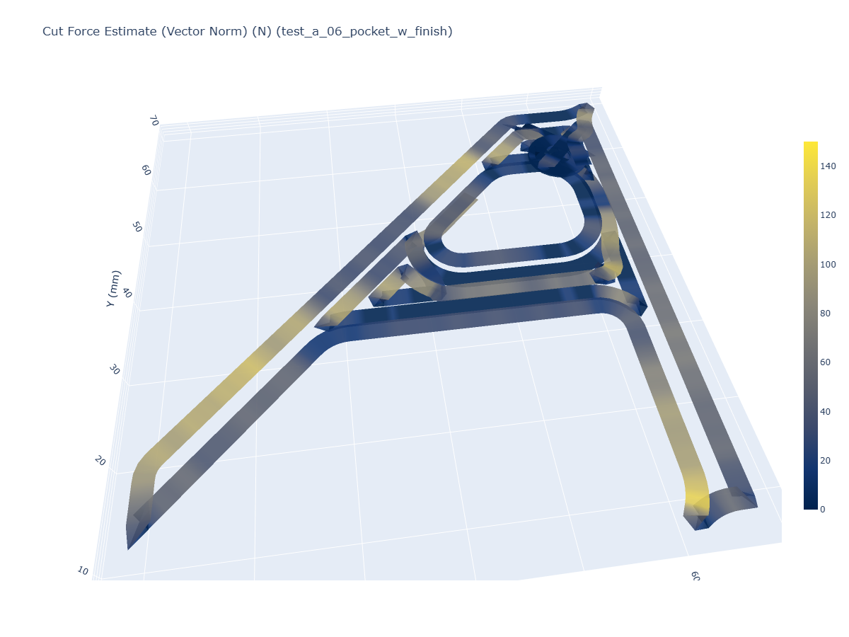
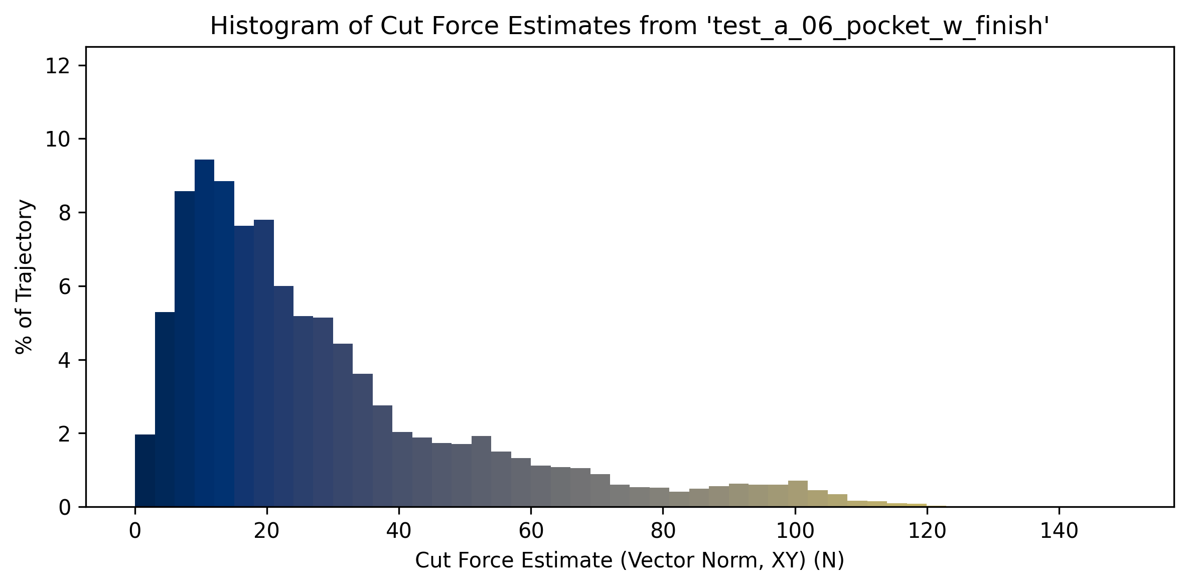
Another note here is that this cornering is done partially during the cut and partially during traverse into the next cut. CAM tools do not calculate cutter engagement area, so it is difficult from those alone to ascertain where in these distributions the velocity deviation may cause issues (if the deviations appear only when we are linking two cuts, they matter only in terms of total part time). In our case, we can combine our cut force estimates with chip load deviations to plot deviations only where our cut force is larger than some value: below I chose \(25N\) as a deadband.
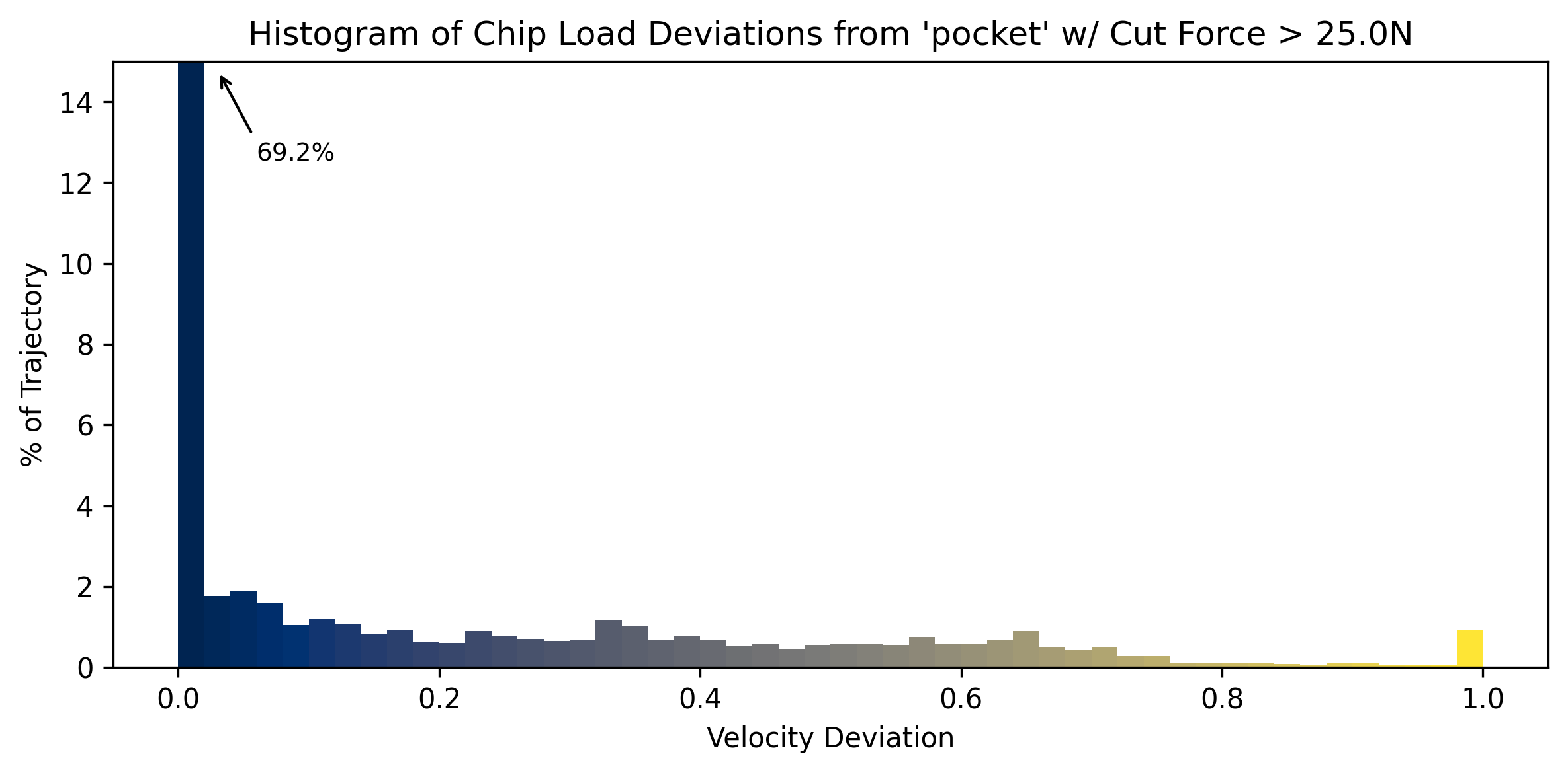
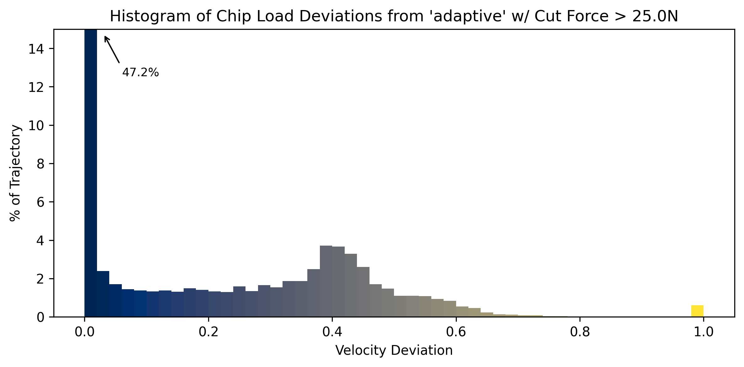
The differences in the distributions above is subtle, but shows us that about half of the adaptive path’s worst deviations (around \(0.4\)) take place in areas of low engagement / low cut force. Finally I will note that the worst deviations in the adaptive path (where there are many corners, but most with some radius) are smaller than the worst in the pocket toolpath (where there are less corners overall, but those corners have sharper angles).
The pocket toolpath was faster overall; a total of \(153s\) of operation. The adaptive path took \(216s\).
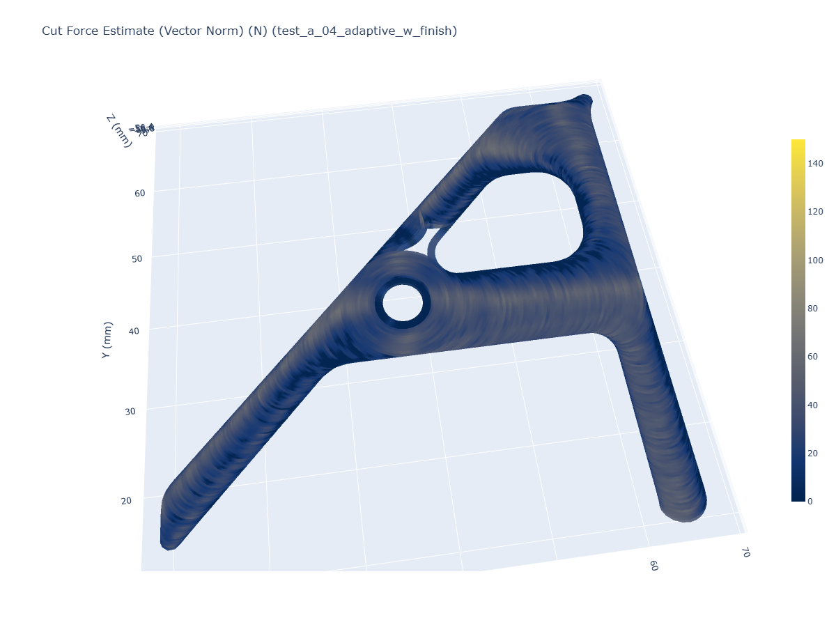
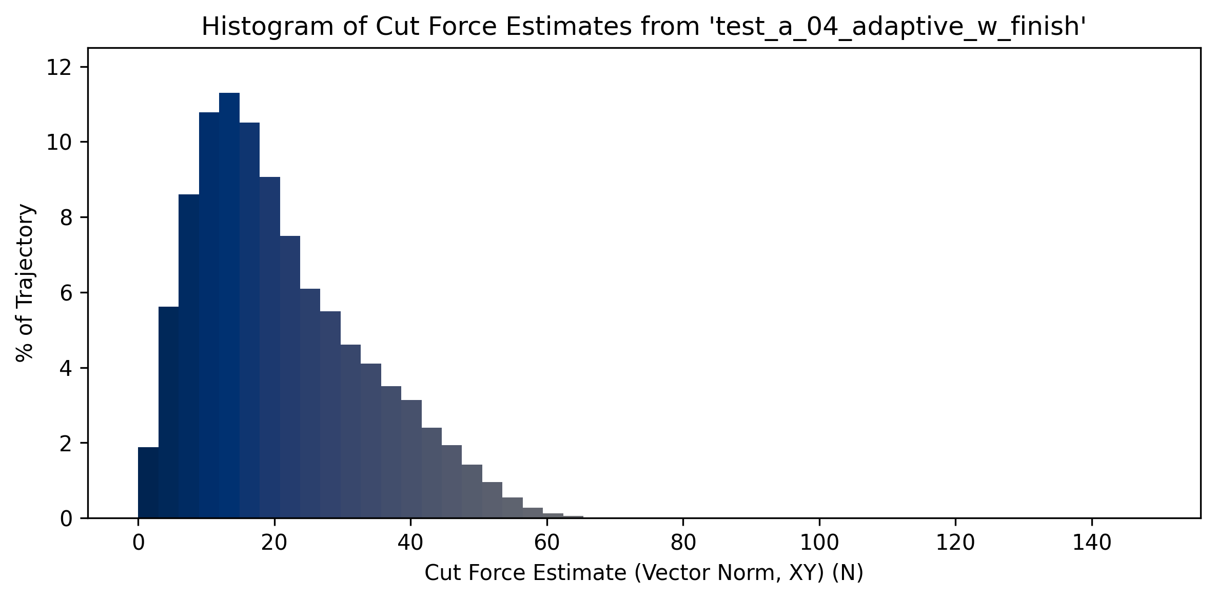
Comparing cut force estimates in both toolpaths provides some more insight as to the strengths and weaknesses of either strategy. In the histograms above, we can see that the adaptive path uses overall lower cut force, and has a much smaller maximum force (around \(60N\)) than the pocket (~ \(115N\)). The 3D plot shows us where these hot-spots are: in the regions where the pocket toolpath must slot, i.e. cut with the full width of the tool. This is the primary weakness of traditional toolpaths: slotting is inevitable in parts with narrow channels to cut, which leads to high variability in cutting loads during machining. Slots also present chip evacuation issues, as the cutter has limited space around it to throw chips.
7.5.5 Model-Fit Quality
It is difficult for me to evaluate the quality of the cutting force model in this chapter, since I do not have any ground truth measurements for machine load. However, I do evaluate the quality of the motion model fits from this experiment and and the printing section (6) in 5.7.2.
7.6 Summarizing Discussion
In this chapter, I showed that basic motor and kinematics models can be used to:
- Help us to design machines (7.5.2), in virtually combining motor and axes faster than would have been possible were we to physically couple and measure each, and in using those models to intelligently select optimal motion control parameters with guarantees (rather than guesses) about those parameters’ feasibility.
- Help us to predict what will really happen when we run our machines (7.4.1), in simulating as-optimized toolpath velocities using our software-defined machine controller.
- Generate new data (cutting force estimates, 7.4.2) that can be used to understand what is happening as we run our machines.
Each of these contributions still relies heavily on tacit knowledge in machine design and in machine operation. The design workflow required heuristic estimates for requirements, i.e. in estimating how much force bandwidth is enough and what types of feedrate will be desired during operation. The machining workflow incorporated tacit knowledge for chip load (and it’s relationship to feedrates and spindle speed), an understanding of how cutter engagement area relates to cut force, and an understanding of spindle limits.
As in the FrankenPrusa (6.4.2), our workflow doesn’t add any new instruments to the machine (besides motors, which are of course required in any configuration), it only modifies control software. This makes progress towards our mentioned goal of retrofitting existing hardware with smarter controllers. I discuss this at more length in Section 8.2.
7.7 Future Work
This work covers only the very basics of what model-based CNC might entail. We want to go towards a more complete workflow, where models enable machinists to make better parts, more rapidly, and where models can help to train new operators.
I think the framework for doing this is clear; we need computational models of our machines, i.e. software objects that can be used to simulate our hardware and its control. These can be inspected at a high level and inform heuristic parameter selection, and (as they are developed) be used to directly optimize pieces of the process. By developing models on the hardware where they are used, we avoid the common issue where models diverge from reality, becoming more troublesome than they are useful.
The CNC industry is old and resistant to sudden change; we cannot realistically propose that we should retrofit everyone’s hardware to accomplish these goals. However, there may be minimal changes available, and much of the modelling work can be useful even at coarse precision within existing workflows.
From where we are at the moment, I would proceed in a few steps.
7.7.1 Predicting Cutting Forces
Cutting models themselves are already very well understood, the challenge in our framework is to fit them with instrumentation available on our machines.
It’s clear that spindle load is a primary limit in many machining systems, stalling spindles is more common than stalling a machine’s kinematics. In the hardware that I developed here I didn’t have time to instrument the spindle, but doing this would have the clear benefit first of understanding its power constraints, but also as a tool to develop cutting force models: the torque required to shear the material apart, at a known tool tip diameter, is probably a key instrument in learning those models. In fact, where realtime feedback is available to CNC operators, spindle load is typically the first to appear, meaning that these data are at least readily available within state of the art machine controllers (but is presented as a simple load percentage - it is measured in amps, as in any other motor model, so the last step is fitting some \(k_t,\) which I expect is well understood by machine and spindle manufacturers).
The primary challenge that I expect in developing cutting models is measuring cutter engagement area - that is, how much of the tool’s surface area is passing through uncut material? This is dependent on the machine’s position in the part (of course!) but more importantly is dependent on the current state of the stock geometry, as it goes from a block to the finished part. Computational representations for constantly changing geometry are challenging; probably the simplest is a voxel space, but the memory required to store 3D voxels quickly becomes punishing as we increase resolution.
These are also highly dependent on variables that frequently change: the average CNC shop stocks hundreds of unique tools, and hundreds of thousands are available in the industry. Each has variable geometry, but also variable surface coatings, etc. Models developed for cutting forces would have to be transferrable across this heterogeneity if they are to pose any practical use, or they need to be easily developed using test equipment available in most shops: i.e. the machine itself.
7.7.2 Intelligently Selecting Feeds, Speeds, and Engagement Areas
If we can predict cutting forces, selecting feeds (linear traversal rates), speeds (spindle RPMs), and engagement areas (stepdown, stepover, etc) is likely an easier task. At a coarse step, this is as simple as writing down ideal chip load heuristics, and then selecting cutter engagement areas such that spindle load and motion system loads do not exceed the machine’s limits. There is a space of these solutions that lie along two degrees of freedom: linear feedrate corresponds directly to an optimal spindle RPM (given a chip load), and total cut area can be framed either with a set stepdown (producing a stepover such that area remains equal) or a set stepover (producing a stepdown …). As I showed in the printing section, we can then apply an heuristic about how hard we want to work: how much proportion of the machine’s underlying limits do we want to deploy in the cut?
The other constraint here (in these selection problems, constraints are helpful) has to do with chatter, which I discussed only breifly in this chapter but is in practice probably the predominant problem that faces practical machinists.
- Chatter occurs when the cutting edge excites the machine / tool / part structural system at its resonant frequency.
- It is a function of three things: frequency response of that system, input frequency (spindle speed x no. flutes), and the cutting force (excitation amplitude).
- Much research on chatter prediction and avoidance exists,
- TODO: stick a chatter stability plot in here, or point to one cc @ Tony Schmitz.
Chatter involves stiffness and frequency response data as exists in the SOTA Section 7.2.4.2. Also involves stiffness of the tool (simple beam bending can help, w/ i.e. factors for flute count). Most challenging of all is that part stiffness changes during the course of the job. Modelling that in a feed-forward manner is challenging but not impossible, it just requires tight coupling between geometric representations and the controller (as already mentioned above for cutting models: voxels are heavy).
It may be more productive to rely on real-time estimates of cutter force (of the kind that I explored here), and known values for excitation (spindle RPM, basically) and the machine and tool’s stiffness - leaving just the part stiffness and damping as free parameters. These change not only as the part becomes smaller, but also when we excite the part from different locations. During operation of one-such chatter detecting machine, we may be able to use a rolling estimate of that excitation to differentiate which direction in the stability plot we are heading (into more or less excitation, which could tell us which direction we need to turn in (RPM, \(v(s)\)) in order to reduce chatter).
This sounds like a good start, but practitioners will note that once you have entered chatter you are already done for, the part may be ruined even if you correct the issue shortly thereafter. This is why predictive models are important. Either we need to model geometry so completely that feed-forward controllers can reliably avoid chatter, or our chatter detection models need to be tuned well enough that they can detect the conditions that arise just before chatter begins.
7.7.3 Intelligently Selecting Tools and Path Strategies
So, if we can manage cutting force models, spindle instrumentation, and chatter, we can probably pick most parameters for any given CNC operation, if we are provided with a tool and a machining strategy - i.e. one of those shown in Figure 7.3.
However, when I have spoken to practical machinists about this project, they cite these early steps (tool selection, strategy selection and ordering, and part fixturing) as their largest burdens for overall productivity. With this framing in mind, I want to proceed to the next topic.
7.7.4 CNC Machining as an Explicit Constrained Optimization Problem
- In this thesis I showed that it is possible to solve machine “speeds and feeds” in FDM, using an online optimization of motion and process via models. This included similar components to those that would be applicable in machining.
- Models we have discussed, the main issue is the geometric representation of the problem.
- It is my expectation that it will soon become possible to solve this problem (and the others) using direct optimization. The computational lynchpin is the geometric representation of the stock being machined, and the memory required to properly represent that as it changes. Luckily for us, GPUs with exceptionally large memories are what the world is hungriest for right now, and they will continue to expand.
- Whereas others approach this problem by looking at datasets of parts and GCode, I think a lower level approach (models and differentiable simulation) is likely to win out: it would be more transferrable across tool and material parameter space, and across the heterogeneity of machines - each with their own quirks.
- It is likely that reinforcement learning should be mixed with lower level approaches, i.e. to learn which areas of a part should be machined first, etc.
7.7.5 Real-Time Thermal Imaging in CNC Machining
I found the thermal camera deviously useful and would anticipate that its inclusion in any to-be-developed instrumented CNC machines extremely valuable (as it is in printing) - perhaps less so where flood coolant is used continuously, but i.e. wood routers and smaller machining centers (where no, or only mist cooling is present) would benefit immensely from this data.
7.7.6 Generating Useful Outputs for Machinists
I want to close the section with a note on the utility of automated systems, and who they are made useful for.
- The goal of completely automating machining is suspect: as in other cases in automation, developers of technology are too eager to replace humans with intelligent systems. Especially in machining, which is filled with corner cases, gotchas, and valueable tacit knowledge that is very difficult to articulate in computational models, we should not make this a primary goal.
- Instead, work on modelling machining is probably most useful (and most immediately useful) in helping machinists to better develop their understanding of the process: to understand cutting physics with models, rather than to develop models that replace their intuition.
References
Many readers will be familiar with High-Speed-Machining, a series of milling strategies developed somewhat recently. These generate tool-paths that effectively minimize cornering radii for the majority of the work that they do. These were a kind of magic when they were introduced, and were realizeable only when modern machine controllers could readily handle the complexity of the instructions produced. It is my intuition that this insight was not so much about maintaining high feedrates, but that the resulting geometries mean that more of the actual milling time is spent at the target feedrate - i.e. tight corners, which produce feedrates lower than those set in parameters, were minimized.↩︎