5 Motion Control with Machine Models

5.1 Chapter Introduction

Earlier I was discussing how machine operation is limited by real-world constraints: motors produce limited torque, structures deflect with load, polymer extrusion is limited by fluid (and thermal!) dynamics, cutting forces are limited by tool and part stiffnesses, etc. Implicit to CAM programming is that users should setup parameters such that their GCodes don’t require the machine to violate these constraints. In real-time machine control (where those GCodes are turned into actual motion) we use velocity planners to limit machine acceleration and avoid violating our machine’s kinematic constraints. This is the hidden optimization that I spoke about in the introduction (1.2.4.1), and it takes place beneath the GCode layer, i.e. in a firmware on the machine’s control board.

In the state of the art, this is done using a type of solver called a trapezoid planner or s-curve generator (depending on who you ask). I explain how those work in more detail below (5.2.1), which are configured using estimated parameters for a machine’s maximum velocity, acceleration, and (in some cases) jerk. However, this approach greatly reduces the dynamic range used by machine actuators during operation and ignores exploitable motion dynamics like damping assymetry (we can decelerate faster than we can accelerate because friction is working with us).

In Section 3.3, I showed how we can bring these controllers up out of machine firmwares and make them into software objects. That roughly solves the problem of the hidden optimization simply be relocating the algorithm into a higher level system where it can be more easily modified and inspected. In this chapter, our main motivation is to see how we might articulate motion control explicitly as a constrained optimization problem, and what benefits that may have for machine operation and machine design.

5.1.1 Methods and Evaluation Overview

This requires a few key methods. Firstly, we need to develop and fit models can will articulate motion constraints. I cover models for electric motors in Section 5.3.1 and for kinematics (transmissions, inertias, and friction) in Section 5.3.2. To fit these models on the hardware where they will be used (5.5), I develop a closed-loop stepper driver and a method for learning some of it’s key parameters automatically (Section 5.4).

In Section 5.6 I develop a motion planner in an optimization framework that uses these models. It has the simple task of maximizing speeds while respecting actuator and kinematic constraints. Doing so with high fidelity models for motion is computationally expensive; I lean on a set of tools that have been recently developed for parallel computing on the GPU, and carefully frame the computation such that it remains parallel in structure (5.6.1). The outline here is that the solver iteratively picks a series of velocities, calculates accelerations required to achieve that series (5.6.1.1), translates those states into actuator requirements (5.6.1.2), and then calculates a cost for that solution (5.6.1.4) (violation of constraints is costly, overall speed is rewarded). The derivative of that cost with respect to those velocities is computed, and an optimizer updates its velocity selections to minimize the cost.

I evaluate this planner against a trapezoid-based solver in Section 5.7.1, showing how this work increases the dynamic range used by our actuators and thus improving overall speeds. I also assess the quality of our models in (5.7.2) and show how they can be iteratively improved using data from real-world machine operation (5.7.3).

The work in this chapter also enables many other contributions that come later on in the thesis. I expand it to optimize process dynamics for 3D printing alongside motion dynamics in Section 6.9, and use it to generate valuable outputs there as well (6.11.2). Methods for motor and kinematic modelling also enable us to analyze design choices for a milling machine in Section 7.3, and generate cutting force estimates for the same (7.4.2).

5.2 Background in Motion Control

“Motion Control” can mean many things, as is true in many other disciplines. Depending on who you ask, it may be the practice of:
- Tuning a servo’s PID¹ Gains to generate smooth and precise response to target positions or velocities.
- Generating single-segment acceleration “ramps” aka trapezoids to smooth motion over longer spans.
- Optimizing motor commands in a bipedal, legged, or 6-dof robotic system,
- Path Planning, i.e. generating trajectories themselves (deciding where to go).
- Etc; in practice robotics, and machine control as a subset, is a mixed bag of all of these activities. In this thesis, Path Planning is the trajectory generation step, and for Motion Control I mean the specific task of Velocity Planning - where we, knowing the path we want our machine to take (our target trajectory), pick the velocities that it should use along that path, generating a planned trajectory.
It is already normally framed as a constrained optimization problem: pick as large of a velocity as you can, subject to (1) some maximum velocity encoded in the trajectory, and (2) our system’s dynamics (at first glance: acceleration, velocity, and jerk limits).
SOTA velocity planners fall mostly into two categories:
- Heuristics-based trapezoid or s-curve planners, which I discuss in 5.2.1, and serve as our main point of comparison because they are what the vast majority of digital fabrication machines use.
- Optimization-based planners, mostly forms of Model Predictive Control (MPC), that use various Quadratic Programming methods to numerically generate solutions. I discuss these in 5.2.2.
The planner that I develop here differs from both approaches in a few key ways, which I will discuss.

5.2.1 Trapezoidal Solvers

Trapezoidal solvers (or s-curve generators) are the most common and practical type of motion controllers that we find in practice, although the exact configuration of most commercially available machines is difficult to study because their controllers are proprietary (2020). In digital fabrication research, where machines are often controlled using open source hardware, trapezoid solvers are the rule. They are very well understood in texts (see 2017, sec. 9.2.2.2) as single-segment solvers (one line) but their extension into multi-segment trajectories involves one or two tricks that I should explain.

Firstly the basics: they work by generating trapezoids in the velocity-time plot, which are s-curves in the position-time plot.

A trapezoid in the $\vec{V}(t)$ (velocity *along* the path, in time) is s-curve shaped in position, and has square edges in acceleration, and infinite impulses in jerk (the third derivative of position). In this plot, I am extracting these states from a basis spline that encodes the trajectory 3.3.2; that encoding smooths the infinite jerk pulse, inserting a small ramp in the acceleration trace.

Trapezoid segments assume fixed acceleration over each component, meaning the kinematic equations can be used, those are below.

\[ \begin{aligned} d = v_it + \frac{1}{2}at^2 \\ d = \frac{v_i + v_f}{2} t \\ v_f = v_i + at \\ v_f^2 = v_i^2 + 2ad \\ \end{aligned} \tag{5.1}\]

Trapezoids are planned by setting a maximum acceleration (slope in $v(t)$) and velocity (maximum value in $v(t)$). Using these values along with initial and final velocities $v_i, v_f$ and a distance for the segment $d$, we can easily generate trapezoids for entire linear segments. Once they are planned, they are also straightforward to encode in data structures in firmware that can be rapidly evaluated as a function of time, to i.e. generate stepper motor pulses or servo target values in a motion controller’s firmware.

Lists of linear segments are linked (choosing cornering velocities) with an heuristic algorithm called junction deviation, which approximates maximum cornering velocity using an imaginary arc segment between the two lines. This step produces maximum $v_i, v_f$ for each segment. Original blog post on the topic is at (2011) for the firmware GRBL (2011--2024), and explained also (here 2018).
Dynamic programming (2024a) is then used to link $v_i, v_f$ across sequences of segments, such that each segment does not (for example) start at a $v_i$ that is too large to be reduced to the next required $v_f$ over it’s distance. This involves computing a forwards pass (ensuring each segments’ $v_f$ is not so large that it is not achievable with the segment’s $a, v_i, d$), and a reverse pass, which is the same computation but from $v_f \rightarrow v_{i,max}$
Each segment is evaluated to see which (of seven) possible trapezoid variants it may produce, and encoded in a manner where it can be evaluated as a function of time. Motion controllers then iterate through these segments, through time, and produce control outputs that cause their motors to track through it.

Trapezoids are linked end-to-end using Junction Deviation, an heuristic for cornering velocities, and dynamic programming. This figure shows a series of trapezoids extracted from a solved trajectory, and their derivatives in time.

It is worth noting in this point is that trapezoid solvers are based on fixed maximum accelerations and velocities, whereas motor dynamics show us that they are capable of more: larger accelerations at low speeds, and higher speeds where low accelerations are required. Where our machines have nonlinear kinematics, minimum and maximum velocities and accelerations change through space as well; a robot arm requires more torque to move its base joint when it is outstretched because the rotational inertia of the arm is larger when it is in a longer configuration. Because trapezoidal solvers are fundamentally based a set of kinematic equations that are based on segments with fixed acceleration over their length, they are unable to exploit this dynamic (unless we chop our line segments into lots of little lines). They are practical, however, for the same reason: entire linear (and arc) segments can be rapidly evaluated with a small number of clock cycles.

5.2.2 Optimization-Based Solvers

State of the art optimization based solvers are typically Model Predictive Controllers (MPC) that are solved using Quadratic Programming (QP) (2002). MPC controllers work in much the same way as you and I do: we use a simulation of the future to optimize future and current control outputs. The classic example comes from driving: when we are entering a corner, we know that we need to slow down before we turn. To pick a braking point, we use a mental model of our car’s dynamics (how long it takes to slow down) to “simulate” (imagine) how long it will take to come to the appropriate entry speed for the corner. With computational MPC, we simulate and optimize control outputs over a horizon of up to a few seconds at each time step, but only issue the immediate next control output to our system. These are common in practice to solve controls problems for legged and bipedal robots (2018), (2016) and i.e. quadcopters (2021). The best practical overviews of their implementation I have found are in (Tedrake 2024b) and (Brunton and Kutz 2022b).

These solvers are constructed symbolically and are subject to the constraint that the optimizations they solve must be quadratic, i.e. highly convex with one global minima. Two common tools for this practice are CasADi [-Andersson2019] and acados (2021). CasADi lets developers author symbolic representations of their system dynamics and cost functions, and then generates C code for evaluating derivatives and integrating dynamics models. Acados is a solver that can directly use those C codes to minimize cost functions in real-time. These are akin to programming languages and compilers: we write systems and constraints at a high level (mathematically), and then automatically generate programs (solvers).

MPCs are typically either formulated using a “direct shooting” method (where the solver picks control outputs over time, some $u(t)$), and then calculates forwards (from some starting state) how the system evolves over time given those inputs. This is perhaps the most comprehensible formulation because it mirrors how we naturally think about dynamical systems. However, it requires serial computation of the system’s evolving states which makes it difficult to compute, and gradients can vanish over long integrals. The other formulation is called “direct transcription,” where the solver picks the resulting trajectory (Tedrake 2024b). This breaks the time dependence and allows us to parallelize much of the computation, but they also require that the solver implicitly link each time state, such that control states at each time $u(t)$ for each system state $x(t)$ generates the next system state $x(t + 1)$. Because the solver is now choosing outcomes as well as inputs, the dimensionality of the problem increases.

As I will discuss, the solver that I develop here is akin to a direct transcription style MPC, but different in two ways, as I will explain in 5.6.1. Using this formulation, rather than describing systems symbolically, I can write models as python functions. Rather than using QP solvers, I write cost functions and then use a generic solver framework (originally developed for the authorship of i.e. LLMs and Diffusion Models) to minimize the cost function with respect to those velocities.

This is significantly less performant than the state of the art in MPC for realtime control in terms of the FLOPs² required (and less deterministic), but simplifies controller authorship and allows us to add dynamics to the system that may be cumbersome to describe symbolically. It also enables us to use the same component descriptions (functions with parameters) in the model fitting and model-based control workflows, and avoid the step where we might re-compile and update a firmware when we generate new models (as in with CasADi and acados). I make up for the increased FLOPs requirement by formulating the computation so that it parallelizes well on the GPU, and developing the low-level motion system description and representation in Section 3.3.

5.2.3 Reinforcement Learning

The headlines in robotic control these days is about Reinforcement Learning, but it is:

Mostly applied to legged or wheeled robots (Disney, RAI),
Mostly done with gradient-free methods,
Mostly done using digital twins as a basis to perform higher level goals-oriented work: we cannot RL if we cannot simulate systems well.
In this framing, this thesis lays the groundwork for us to enable RL-type controls at higher levels in the stack, i.e. in path planning for machines (CAM, slicers), a domain that I do not engage with besides in discussion.

5.2.4 Integrating Optimization-Based Solvers with Machines

MPC is common in robotics but less so in machine control, although it has certainly been developed, i.e. in (2022), (2016). Again, it is impossible to know how common these are in deployed industrial equipment (2020). I often find papers in machine control where the authors have developed new control algorithms for i.e. milling or printing, but are either unable to deploy those algorithms (using simulations to verify them), or deploy them by having their algorithms write custom GCodes that are then interpreted by machine controllers. The two references above are both cases where this is true, and in (2021) (probably the most complete MPC implementation on a CNC machine that I have found), the controller is implemented using GCodes alongside live-updates to the machine’s feed override and spindle RPM settings. This allows the authors to modify the machine’s own velocity controller’s setpoint, but not bypass it entirely - they take steps to model that controller’s own response in order to properly develop their intervention³. In fact, that author later finished his PhD on the prediction and modelling of GCode interpreters themselves (2022) for the purposes of developing these types of “piggyback” control systems for CNC machines. In (2008), explicit mention is made of the challenges this poses: “… The actual feedrate is thus locally lower than the programmed on due to the interpolation cycle time.”

This explains the second important difference between this work and others, which is that the controller described here is integrated more directly into the hardware that it is controlling. This is a result of the work from Chapter 2 and Chapter 3, which provide the frameworks required to easily connect new controllers to hardware.

5.2.5 Constrained Optimization and Differentiable Simulation

I am enabled to complete the work in this chapter largely because of a new availability of automatic differentiation (aka autograd) tools, that automatically generate gradients for any given program (gradients being a key ingredient for optimization, most performant optimizers are based on gradient descent). In particular, I am using JAX (2024). With JAX, any system that can be articulated as a purely functional python code can be automatically differentiated. We can then use the function’s gradient to optimize the function’s inputs, and JAX conveniently pairs with optimizers from the OPTAX library (2024). The performance of this system is only viable because JAX also includes a just-in-time compiler that turns the whole system into code that can run in parallel on high performance hardware (i.e. a GPU).

MPCs are typically used for short-order optimizations, operating over time horizons around one to five seconds. They usually run somewhere between 50Hz and 500Hz since the compute required to solve them is intense. For longer horizons of control, the current best practice uses simulated systems to train policy controllers (2022a) that can issue higher-level control commands. Policy controllers are normally coupled with lower level, faster feedback controllers and classical controls components like kalman filters and PIDs. (Kaufmann et al. 2023) is a particularely clear example of how all of these components come together to produce performant controllers. Policy controllers are often trained without gradients because it is hard to differentiate across long time spans, but recent work deploys differentiable simulation to overcome this issue (2024).

All told, optimization based control is a vast, complex discipline. I have not mastered any of it, but the available tools have become sophisticated enough that I can generate a solver using my own models and deploy it in practice. Above all, this is a testament to the community of researchers and engineers working together to advance the practice, who are committed to sharing reproduceable, useful tools with one another.

5.2.6 The Role of PIDs and Hierarchical Control

Controllers of any complexity are normally formulated hierarchically, where lower levels (like current control) are handled with simple i.e. PI controllers (no derivative term), and more complexity is added as we move up in systems scope and down in response time, see (1980), and (2014) or (2023) for modern hierarchichal systems.

The rule of thumb is that the bandwidth of the controller below the one you are currently designing should be fast enough that the delay it introduces can be ignored when compared to the current level. A good example of this comes up in Section 5.4, where I develop a motor controller that uses two levels of control (microseconds and milliseconds) that subsequently plugs into the velocity controller from this section 5.6, which spans seconds of motion.

5.3 Models for Motion Control

This section covers background on key models for motion, for motors (below) and for kinematics and damping (5.3.2). I then use a closed-loop stepper driver (5.4) to fit those models to data in Section 5.5.

5.3.1 Motor Models

Motor physics are the most foundational for motion planning: as discussed, we need to understand these physics to know what our motion constraints are going to look like. This means electric motors in their many forms: classically we have Brushed DC, more modern control typically happens on Brushless DC (BLDC or PMSM: Permanent Magnet Synchronous Motors) which both rely permanent magnetic fields interacting with changing magnetic fields, and Induction or Reluctance motors, which operate based on the field’s propensity to “want” to move through magnetic circuits that have low reluctance. Luckily for us, the models are all very similar and basically involve generating current with voltage, and then figuring out how current (which is a close proxy for magnetic field strength) relates to the motor’s torque and speed.

Because they are extremely common in machine control, I take particular interest in Stepper Motors, which are known technically as Hybrid Permanent Magnet Reluctance Motors. They work partially like a BLDC and partially like Reluctance Motors.

A dissassembled Stepper Motor, showing the stator with windings (copper) and teeth (steel laminations). At left, the rotor on its own showing the tooth offset on the top and bottom laminations - the biasing permanent magnet is in between those.

Our motor has a stator (the static part) with electromagnetic windings that can generate a magnetic field, and a rotor that has a permanent magnetic field. Motors work because these two fields (in the stator and rotor) want to line up with one another (which is a way of saying that they are in a lower energy state when they are aligned). The teeth in a stepper motor are arranged such that these aligned states are closer together: given some stator field, the closest alignment for the rotor is never more than $7.2^\circ$ away from the rotor’s current position. That is, for every electrical rotation, when we rotate the magnetic field through $0, 2 \pi$ only $1/50^{th}$ of a mechanical rotation occurs.

When the motor is operating, we switch current in the stator to motivate the rotor to rotate continuously. In brushed DC motors, this happens mechanically: the brushes are aligned such that any current passing through them switches onto the windings that will generate current out of phase with the rotor. In brushless motors (steppers are one type of brushless motors), we do this using digital switches and some computing. This process is called commutation in all cases.

The motor physics for any electric motor breaks down into a few constitutive equations, which are below: the electrical half of the motor in 5.2, the mechanical equations in 5.3, and a table of each symbol, its units, and meaning in 5.1.

\[ \begin{aligned} Z &= \sqrt{R^2 + (\omega_e L)^2} \\ \omega_e &= \omega_m p \\ V_p &= V_a - k_e\omega_m \\ \dot{I} &= (V_p - RI) / L \\ I_{ss} &= V_s / Z \\ \end{aligned} \tag{5.2}\]

The electrical half of the model describes how the voltage that we apply to the windings $V_a$ becomes the rotor current $I$ which will generate torque. The first equation above define’s the motors impedance: $Z, \ ohms$ - this is important especially in stepper motors where inductance $L$ can be quite large, and is one half of the reason that generating current at high RPM’s is difficult: with very many pole pairs $(p)$ in a stepper motor (50), we quickly end up with large impedance in the stator when we get going at high speeds. The second equation shows how electrical and mechanical speeds are defined by pole pairs.

The third, fourth and fifth lines above describe stator current. We have that the voltage potential across the stator windings - $V_p$ - is the applied voltage less back-EMF $(k_e \omega_m).$ Back-EMF is the voltage that the rotor generates as its magnetic field moves through the stator’s windings.

The dynamic value of the stator current $I$ is defined by its rate of change (fourth statement): $\dot{I}$ is potential voltage less voltage already contained in the stator $(RI)$, divided by its inductance. This is the term we want to use if we want a time-varying estimate of current, or to estimate the maximum $\frac{dI}{dt}$ which becomes common later on in this chapter. In steady state (fifth statement), this current is just the potential voltage divided by the speed-varying impedance.

\[ \begin{aligned} Q &= k_tI \\ \dot{\omega_m} &= (Q - k_d\omega_m) / J \\ \Theta &= \smallint \omega_m \, dt \\ \end{aligned} \tag{5.3}\]

The mechanical half shows that torque generated by the motor $Q$ is a simple multiplication of stator current with the magical $k_t$ parameter (which we will fit to data later on). The rotor acceleration $\dot{\omega_m}$ is torque, less the torque produced by rotor friction $(k_d\omega_m)$ divided by the rotor inertia $J,$ and the rotor’s angular position is just the integral of mechanical speed.

Table 5.1: Table of motor model symbols, units and values, including notes on how the motor controller in this chapter 5.4 interacts with them.

Symbol	Units	Value	Source ?
$V_a$	$Volts$	Voltage applied to the stator coils	Output(t)
$V_p$	$Volts$	Voltage potential at the stator coils	Product(t)
$A$	$Amps$	Current in the stator coils	Measurement(t)
$R$	$Ohms$	Stator’s DC Resistance	Measurement
$L$	$Henries$	Stator’s DC Inductance	Measurement
$Z$	$Ohms$	Stator’s Impedance	Product(t)
$\tau$ (tau)	$Nm$	Torque	Measurement(t)
$p$	n/a	Number of Pole Pairs	Measurement
$\omega_e$ (omega)	$radians/s$	Rotor Electrical Velocity	Product(t)
$J$	$kg \cdot m^2$	Rotor Inertia	Measurement
$\Theta$ (Theta)	$radians$	Rotor Angle	Measurement(t)
$\omega_m$ (omega)	$radians/s$	Rotor Mechanical Velocity	Product(t)
$\dot{\omega}$	$radians/s^2$	Rotor Acceleration (derivative of omega)	Product(t)
$k_t$	$Nm/Amp$	Torque Constant	Model Fit
$k_e$	$Volts/rad/s$	Back-EMF Constant	Model Fit
$k_d$	$Nm/rad/s$	Rotor Damping (friction)	Model Fit

Two more notes on this, which are not required reading:

The sign of $I$ can easily be opposite to the sign of $V_a$, i.e. the motor is generating current in one direction while our controller is driving it in the opposite direction. This is where electric motors enter regeneration. This is very cool and useful when we are in a battery powered system (renegeration simply shows up as a lift in voltage on the supply, which charges the battery) but can cause issues where we use wall-supplied switching power supplies: they shutdown when the voltage at their output terminals rises substantially past their target output voltage. To ameliorate this, I simply mount a big bleed resistor to my power supplies to perpetually drain excess power (one is seen in Figure 4.20). Done properly, we use a switch across this resistor that only opens when the voltage rises above some threshold - that prevents us from spending energy to make the resistor hot.
By the magic of SI units, the values of $k_t$ and $k_e$ are equivalent (although they have different physical meanings and units). One way to intuit this is that they both describe the interaction between the rotor and stator’s magnetic fields: $k_t$ tells us ~ how much the stator’s field pulls on the rotor’s field, and $k_e$ tells us ~ how much the rotor’s field drives voltage in the stator’s windings. For a better explainer on that topic, see (n.d.).

Most of these values can be easily measured in the real world: $R$ is a simple multimeter test, and $L$ can be measured using an LCR probe. $V$ and $A$ are measured in the motor controller’s firmware, $\Theta$ (and its derivatives for velocity $\omega_m$ and acceleration $\dot{\omega_m}$) are also measured in firmware (using an encoder and kalman filter). Rotor Inertia $J$ is typically included in a motor datasheet, but I have at times taken motors apart to weigh and measure this when datasheets seem untrustworthy. That leaves $k_t, k_e$ and $k_d$ to fit computationally, which we will see later.

5.3.2 Kinematic Models

Except in some rare cases, motors don’t drive machine components directly. They are connected via belt drives, leadscrews and ballscrews, gearboxes (etc) or combinations of each. Understanding the machine’s kinematics enables us to translate between the machine motion we are interested in controlling and the motor models that constrain that motion.

Kinematic models for machines and robots are typically described as rigid bodies connected in kinematic chains using Homogeneous Transformation Matrices (HTMs). These encode translations and rotations. Their effects can be combined by multiplying matrices along the kinematic chain, and to invert a transform we simply take that HTM’s inverse, kind of tautological. Parallel kinematics can be more difficult to describe with HTMs, but we can normally simply pick one side of the parallel mechanism to model.

In this thesis, I wanted to use simpler kinematic descriptions that could easily be articulated as code. For machines, these are also often all we need. In fact for linear kinematic systems we can mostly get by with only the inverse kinematics. I describe these as simple python functions, an approach that is shared by Gestalt (2013) and is common also in open source machine control firmwares (where functions are instead written in C! (2011--2024) (2012--2024)).

So, to start with the model formulations I use here, we have a vector of actuator positions $\vec{X}_{actu}$ and positions in cartesian space, $\vec{X}_{cart}$. For any given machine system, we have a function that describes there inverse kinematics - from the cartesian position to the actuator position. Generically, this is just:

\[ \vec{X}_{actu} = f_{IK}(\vec{X}_{cart}) \]

Importantly for our models, $\vec{X}_{actu}$ units are in $radians$ and $\vec{X}_{cart}$ units are in $meters.$ We will be looking at two systems in this chapter and the next two, one is a CoreXY based FFF 3D Printer and the other is a (kinematically) simple milling machine, their kinematic functions are below.

Listing 5.1: Inverse kinematics definition for the FrankenPrusa (6.4.2).

rads_per_m = np.array([
    -1.0 * (2.0 * np.pi) / 0.032, # a, b: 32mm travel per rotation
    -1.0 * (2.0 * np.pi) / 0.032, # also: inverted, 
    (2.0 * np.pi) / 0.008,        # z: 8mm per rotation 
])

def cart_2_actu_corexy(xyz):
    abz = np.array([
        (xyz[:, 0] - xyz[:, 1]) * rads_per_m,
        (xyz[:, 0] + xyz[:, 1]) * rads_per_m,
        (xyz[:, 2])             * rads_per_m, 
    ])

    return abz

Listing 5.2: Inverse kinematics definition for the CNC milling machine in (7.5.1).

rads_per_m = np.array([
    (2.0 * np.pi) / 0.008,  # x, y: 8mm travel per rotation 
    (2.0 * np.pi) / 0.008,  
    (2.0 * np.pi) / 0.004,  # z: 4mm per rotation 
])

def cart_2_actu_mill(xyz_cart):
    xyz_actu = np.array([
        xyz_cart[:, 0] * rads_per_m,
        xyz_cart[:, 1] * rads_per_m,
        xyz_cart[:, 2] * rads_per_m
    ])

    return xyz_actu

We need to add friction to these models. I use an approximation for Coulomb friction that I will call $Fc(v)$ that combines a viscous term $\mu_{f,v}$ that increases linearly with speed, with an offset term $\mu_{f,static}$. The output from this model (defined with 5.3) is shown below in 5.1.

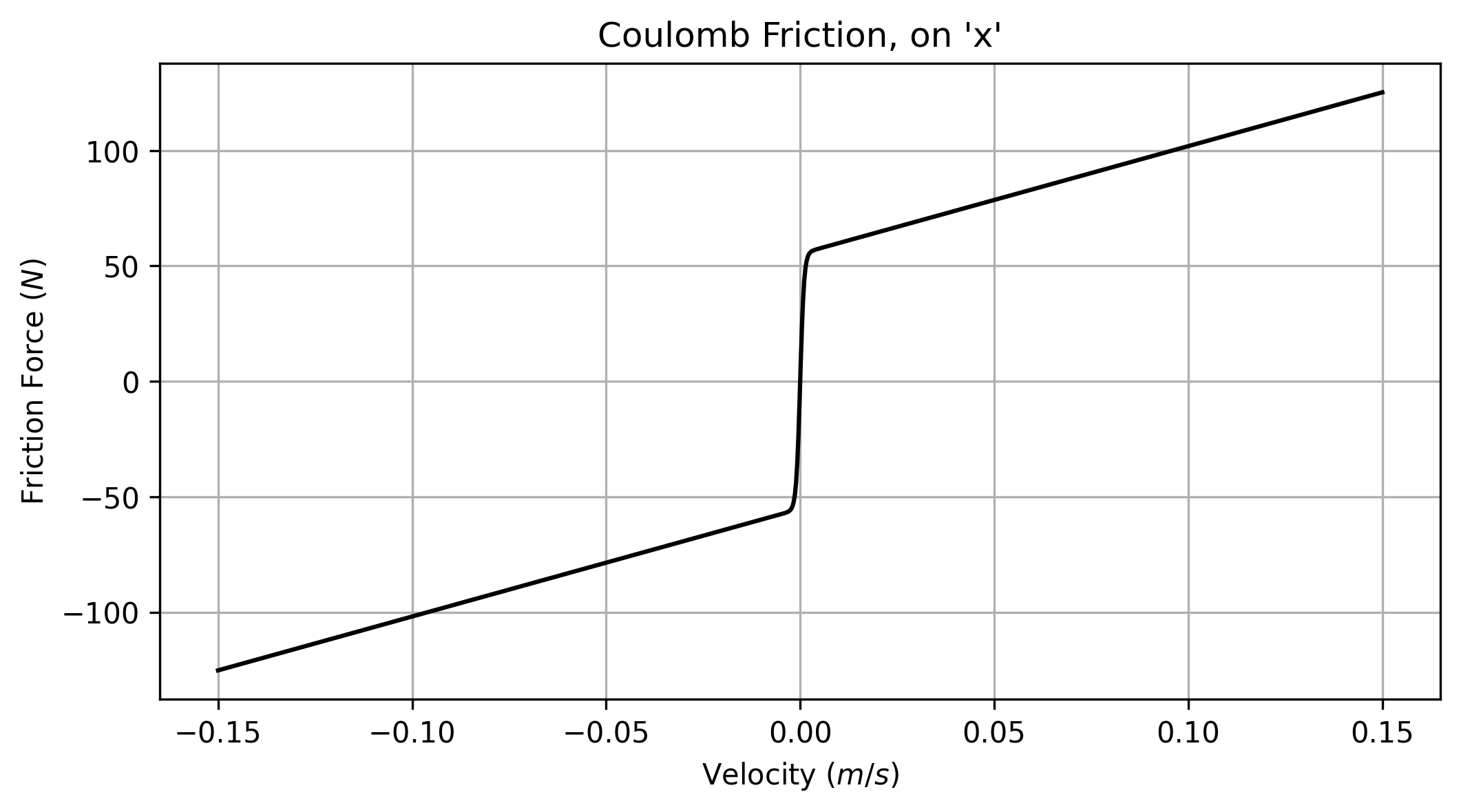
Figure 5.1: Coulomb Friction, rendered with parameters from the x-axis on the milling machine in this thesis. I use `tanh` to smooth discontinuities in the model’s derivatives near the origin.

Listing 5.3: The coulomb friction model as implemented in python.

def coulomb_friction_force(offset, slope, speed, smooth_interval=0.001):
    """
    returns force (N or Nm) of resistance, given speed (m/s or rads/s) input
    offset=(N or Nm), slope=(N/m/s or Nm/rads/s)
    smooth_interval= band of values on either side of the origin (your units) where *tanh* is active. 
    """

    return np.tanh(speed * (1.0 / smooth_interval)) * offset + slope * speed

We also need inertias. I measure these in $kg$ for axes and $kg \cdot m^2$ for rotary bodies (namely motor rotors and leadscrews and couplers in the CNC machine). Using those, we can develop an inverse model that predicts the current required to drive our machine given any velocity and acceleration state at its tool tip.

\[ \begin{aligned} \vec{F}_{req,cart} &= \vec{A}_{cart} \cdot m_{cart} + Fc(\vec{V}_{cart}) + 9.8 \cdot m_z \\ \vec{A}_{actu} &= f_{IK}(\vec{A}_{cart}) \\ \vec{Q}_{rec,actu} &= f_{IK}(\vec{F}_{req,cart}) + \vec{A}_{actu} \cdot a_J \\ \vec{I}_{req,actu} &= \vec{Q}_{rec,actu} / a_{kt} \\ \end{aligned} \tag{5.4}\]

Above, how I combine machine kinematics $f_{IK}()$ with known system states $\vec{A}_{cart}, \vec{V}_{cart}$ and a damping model $Fc(v)$ to estimate required current for the CNC milling machine. In this model we have damping terms on the cartesian system, but not on the actuator system, because those parameters would be degenerate if we tried to fit both sets. Instead, we just fit one set of damping terms, which is sufficient since damping of the motors is directly proportional to damping in the cartesian system: the one term effectively captures both. Below is a similar formulation, for the 3D printer.

\[ \begin{aligned} \vec{F}_{req,cart} &= \vec{A}_{cart} \cdot m_{cart} + Fc(\vec{V}_{cart}) \\ \vec{A}_{actu} &= f_{IK}(\vec{A}_{cart}) \\ \vec{V}_{actu} &= f_{IK}(\vec{V}_{cart}) \\ \vec{Q}_{rec,actu} &= f_{IK}(\vec{F}_{req,cart}) + \vec{A}_{actu} \cdot a_J + Fc(\vec{A}_{actu}) \\ \vec{I}_{req,actu} &= \vec{Q}_{rec,actu} / a_{kt} \\ \end{aligned} \tag{5.5}\]

These both work in a similar manner. First we calculate the force required to move the cartesian system around, which is just $F=ma + F_f$ we then take cartesian states and transform them to actuator states: for linear kinematics, we can use the same $f_{IK}()$ to transform velocity, accelerations, or forces (so long as we use SI units). We add to the required torque $(\vec{Q}_{rec,actu})$ the requirement for spinning the motor rotor and (in the case of the 3D printer, where rotor velocity is not a 1:1 combination of one axis’ cartesian velocity), we fit a set of damping terms in the actuator space as well. Current estimation is then simple, dividing required torque by the actuators’ $k_t$.

5.4 FOC on (almost) Any Stepper

Developing this Field-Oriented Control (FOC) stepper motor was a key enabler of the research in this thesis. I wrote a good deal of it up in a blog post (2025), but will repeat the relevant details here.

Stepper motors are ubiquitous and available in a heterogeneity of form factors at low cost.
They are typically controlled in an open loop manner, where a current controller (normally a chopper driver) cycles stator currents through microstepping tables to move the rotor. It is assumed that the motor rotor will follow $90^\circ$ within the stator current in these cases: when it does not we “miss a step” and the positioning in the system is lost.
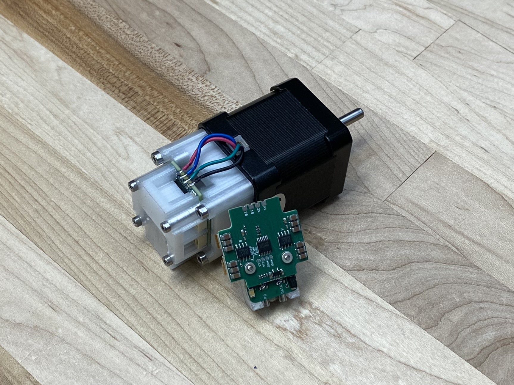
This circuit (and others like it which are available in open source) drive the motor in the same manner that BLDC’s are driven, with closed-loop commutation, positioning, and current control.
The circuit uses a SAMD51 microcontroller, two DRV8251A H-Bridges (which integrate current sensing hardware) and an AS5047P magnetic encoder. The encoder is contactless, and reads field direction from a diametrically magnetized disk that can be attached to the rear shaft of a stepper motor. This, alongside an encoder calibration and model fitting routine, allow us to transform most steppers into closed-loop motors.
Key limits to performance are the SAMD51’s processing power (which is nearly entirely used up in controls interrupts, required to commutate the motor quickly through its very-many electrical phases), and the DRV8251A’s drive power: in practice they saturate around 2.5A of output current.

Figure 5.2: The motor driver I developed in order to complete the work in this thesis. The board can be mounted onto “almost any” stepper motor with the small addition of a diametric magnet being attached to the shaft.

The key ability of this driver for the work in the thesis is that we can measure the amplitude and direction of the stator current, alongside the position of the rotor. The amplitude of the current that is projected on the quadrature axis of the rotor is equivalent to the $a_I$ (actuator current) value in our motor and kinematic models. Measuring this directly enables us to characterize the motors’ $k_t.$ We can then use $k_t$ alongside the current measurements as an estimate for the forces that our actuators are exerting on machines, which forms a basis for kinematic model fits, and some parts of the flow model fits in Chapter 6.

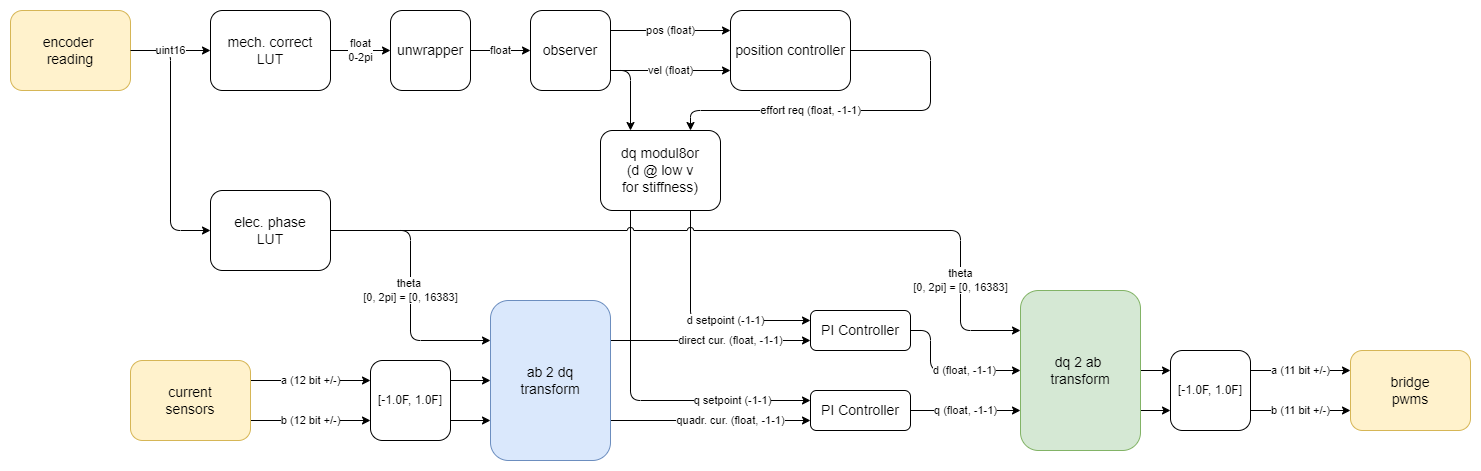
FOC is a controller framework applicable to all manner of electric motors. The algorithm is laid out below (5.3). I relied heavily on Dave Wilson’s excellent blog posts and videos on the topic (Wilson 2015). Steppers differ from most other electric motors with their high pole count (50), which means that our encoder needs to be carefully calibrated such that we can read rotor angle with respect to the stator’s electrical angles precisely. Steppers also must be commutated at much higher bandwidth for the same reason.

The controller implements a Kalman filter (1960) (2006) to estimate rotor position, velocity and acceleration. The rotor is controlled hierarchichally. FOC forms a basis for current control in the stator, using two PI controllers that write PWMs to the driver’s H-Bridges, and sense current in each. The control itself is done in a reference frame that rotates with the rotor - this prevents the controller from having to track rapidly oscillating sinusoidal commands. One layer up, the controller implements either a second PI controller for velocity control, or a PID controller for position control. The velocity and position controllers can be configured to be controlled directly, or with the output of a MAXL spline interpolator.

Figure 5.3: A diagram of the FOC control algorithm as implemented on the motor driver.

The driver’s control parameters can all be read or written remotely. Besides the encoder calibration (which is loaded into firmware at compile time as a lookup table), all of these values are remotely updated when systems are initialized.

Using PIPES, the driver can stream internal control states back to data collectors and controllers. A short list of the most important states in that stream are listed in 5.2 below. States are collected at once, and the bundle of them is timestamped so that the exact measurement time can be reconciled with other system states.

Output	Units	Value
timestamp	$rads$	Time (system $\mu s$) of measurement
encoder_raw	$int$	Raw encoder reading (14 bit)
maxl_position	$rads$	Position from the interpolated MAXL Spline
maxl_velocity	$rads/s$	Velocity from the interpolated MAXL Spline
maxl_accel	$rads/s^2$	Acceleration from the interpolated MAXL Spline
maxl_jerk	$rads/s^3$	Jerk from the interpolated MAXL Spline
obsv_position	$rads$	Kalman estimates of (unwrapped) angular position
obsv_velocity	$rads/s$	Kalman estimates of angular rate
obsv_accel	$rads/s^2$	Kalman estimates of angular acceleration
vcc_rails	$Volts$	Measured voltage on the supply lines
vcc_d	$Volts$	Voltage applied on the $d$ axis
vcc_q	$Volts$	Voltage applied on the $q$ axis
cur_cmd	$Amps$	Target current written by the position or velocity controller.
cur_d	$Amps$	Measured current on the $d$ axis
cur_q	$Amps$	Measured current on the $q$ axis

Table 5.2: Motor motion states that can be transmitted via PIPES at runtime.

The FOC’s PI controllers have gains, which we can set directly via the motor’s $R$ and $L$: this method is also from (2015).

\[ \begin{aligned} k_{p,PI} &= R \\ k_{i,PI} &= 2\pi f_c \cdot L \\ \end{aligned} \]

An important detail to note is that the motor’s PID gains (or PI gains for the velocity controller) must be tuned by hand. I discuss this shortcoming in 5.8.5.

5.5 Fitting Motion Models

Given the models from 5.3, and our motor above, this section describes how I fit free parameters (and which ones I simply measure directly).

5.5.1 Fitting Motor Models

Table 5.1 renders the motor model parameters, and denotes which of these are measured directly (labelled Measurement) or measured by the controller and available as time-series measurements or easily calculated products of other measurements (labelled Measurement(t), Product(t)).

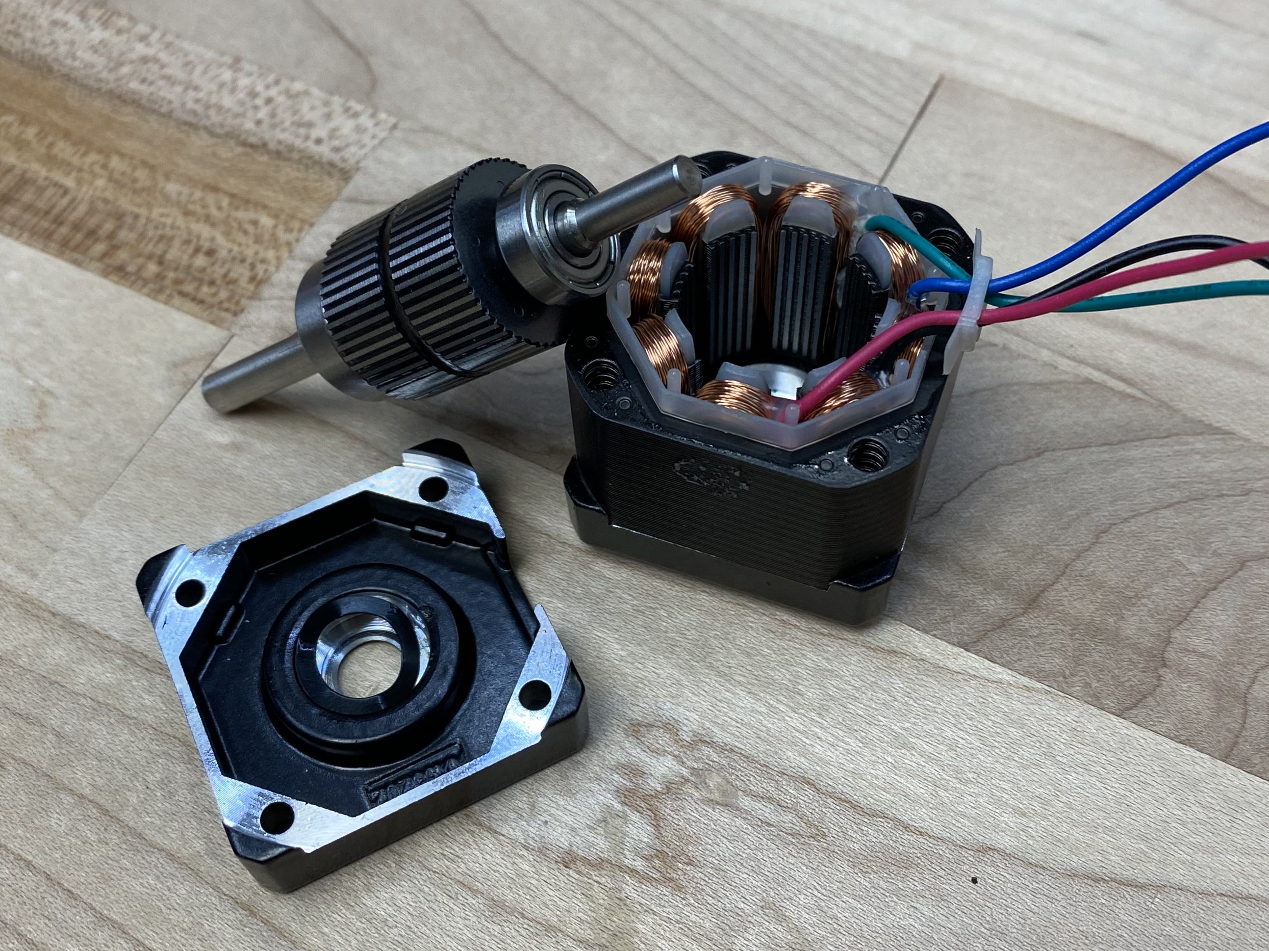
Measurements of static values are often straightforward. I measure $R$ and $L$ with an off-the-shelf LCR probe, the pole-pair count $p$ is always $50$ for stepper motors (and easy to count otherwise). The rotor inertia $J$ can be measured, but only by dissassembling the motor, taking dimensions of the rotor, and weighing it. This is cumbersome, and so I rely often on motor datasheets to include this value. In 5.8.5, I discuss how it is possible to add estimation of these parameters to this step.

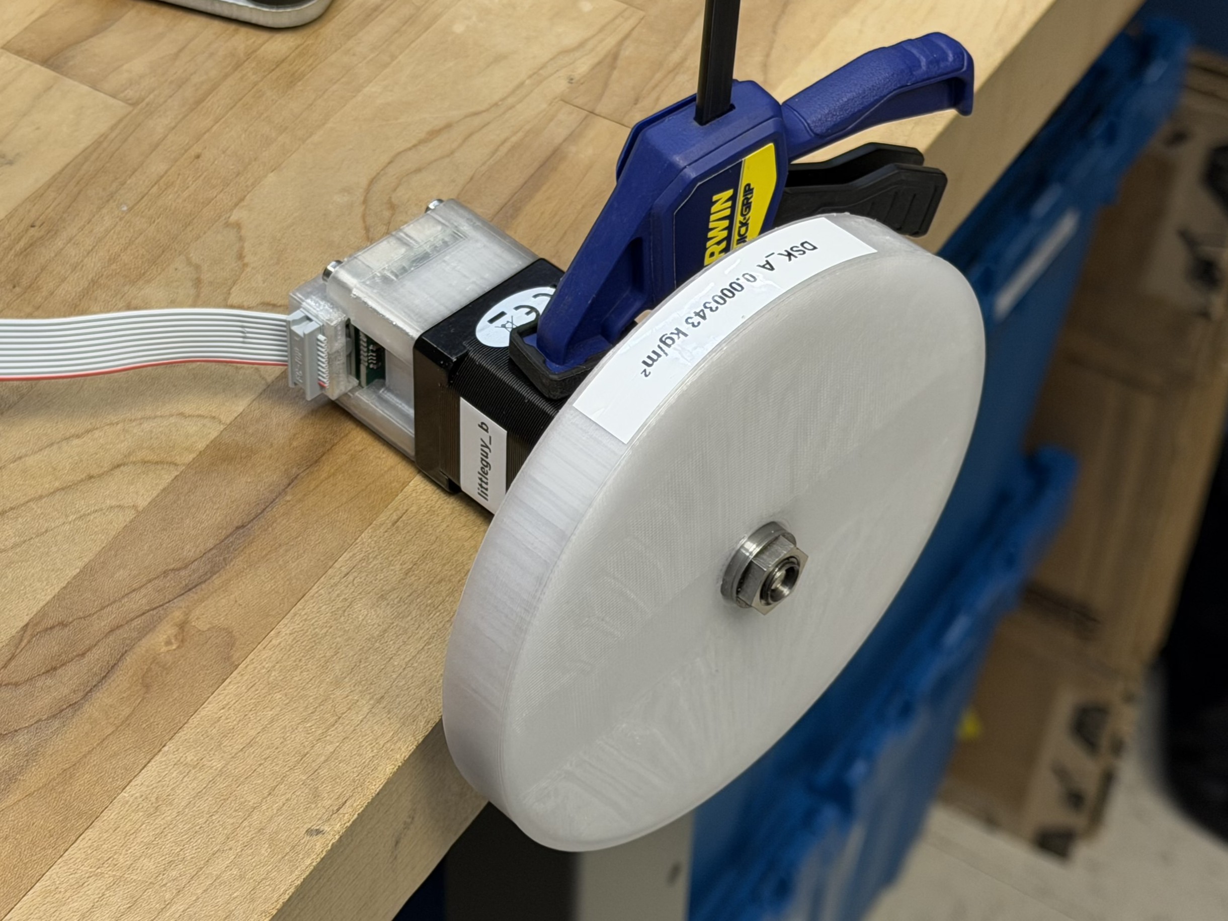
However, that is for later. Here, we make them manually. Then we are left with the three “key” model parameters, $k_t, k_e, k_d$. To estimate those, I developed a simple program that runs the motor in a direct current mode at a number of pre-determined current targets, each for a period that is long enough to get the rotor up to its steady-state velocity (where damping and back-emf overcome the motor/driver’s ability to generate current). I run this program with the motor fixed on a desk, and mounted to a flywheel whose inertia has been measured.

The FOC-Stepper mounted to the desk and attached to a disk with a known inertia.

Test data stores all of the values output by the motor in Table 5.2 in time-series, as well as the test parameters. We can then reconstruct this time-series and fit our model against it.

I do this in two steps, using python and scipy’s optimize routine (1997), (2020). First, we can fit the mechanical parameters $k_t, k_d$ using the motor’s measurements of its velocity, acceleration and stator current:

\[ A = (k_tI - k_d\omega_m) / J \\ \]

Parameters are minimized against a cost function that compares parameters’ acceleration estimates (from above) against acceleration measurements from the motor data, using sum squared error. The motor/actuator’s rotor inertia $J_a$ was manually measured previously, and is combined with the inertia of the test flywheel for this step. The flywheel does two things that are valuable here: (1) it increases the time that the motor spends accelerating and decelerating, increasing data availability in high acceleration, high current (at low velocity) states and (2) it has much more inertia than the motor rotor, reducing overall error that may come from a rotor inertia estimate error since its contribution to inertia is so large compared to the motor rotor itself.

To improve the fit, I also weight measurements by their distribution in velocity. This is useful because most measurements are taken when the motor is at it’s steady-state (terminal) velocity, but we want to ensure the fit is equally biased across velocity states.

def model_kt_kd(params, q_current, vel):
    kt, kd = params 
    accel = (kt * q_current - kd * vel) / J 
    return accel 

def loss_kt_kd(params, cur_data, vel_data, acc_data):
    acc_guess = model_kt_kd(params, cur_data, vel_data)
    return np.sum(np.square(acc_guess - acc_data) * weights)

I estimate $k_e$ separately, despite my note earlier 5.3.1 that the values for $k_t$ and $k_e$ should be the same. This is a bit of a hack, but is a valuable step because we can use this parameter to encode some more information about the motor and controller - that is, that the controller’s commutation is not perfect and introduces a small amount of phase lag. When it sets voltage on the HBridge’s PWMs, those voltages take some microseconds to be actualized in the drive. During those microseconds, the rotor continues spinning. This means that at high RPMs, it seems as though we have more back-EMF, that is, applied voltage becomes less effective.

Fitting this is similar, the model estimates the current measurement given the rotor velocity, some estimated $k_e,$ and the voltage applied on the $q$ axis. The estimated current is compared to the measured current, making a sum-squared error, which is used to fit the parameter using scipy’s minimize routine.

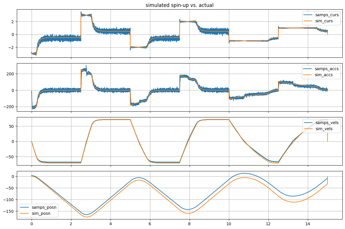
To verify that models explain the motor system, we can plot time-series data against a simulated system, where the recorded control input (a target current) is used to drive the simulation.

Simulation (orange) and data (blue) of time-series data from our model and motor during a “spin up” test.

Models can also be used to generate torque curves across a range of driver setpoint currents, as below:

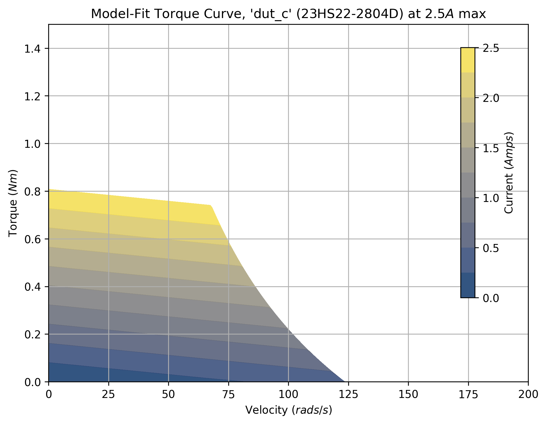
Figure 5.4: The torque curve from a motor-model fit (left), and the motor (right).

Limit to torque generation in these models comes from two places. Firstly, the driver’s current limits (or current setpoints) saturate. Above, you can see that the motor’s torque is limited to $0.8N$ at zero velocity, simply because we cannot drive more than (in this case) $2.5A$ through the driver’s H-Bridges. In practice this limit can be set also due to thermal limits in the motor. As the motor comes up to speed, current generation is limited by back-EMF and the motor’s impedance, which grows as speed increases.

The torque curve is an excellent tool and they are commonly used by machine designers to select actuators, for example if we know that an axis of our machine will mostly be responsible for fast accelerations at low speeds, we will pick a motor with more torque “in the low end,” whereas if we have a large gear ratio and need our motor to work at large RPMs, we will look for motors where the torque does not fall off drastically as speed increases. In Section 7.3.1, I show how we can combine motor and kinematic models to virtually test multiple combinations of each to pick motors using data from our hardware (rather than datasheets), and select velocity controller parameters (for trapezoidal solvers) using the same.

5.5.2 Fitting Kinematic Models

Fitting kinematic parameters follows a similar pattern.

System inertias $a_J, m$ are measured manually.
Inverse kinematics $f_{IK}()$ are written down as python functions.
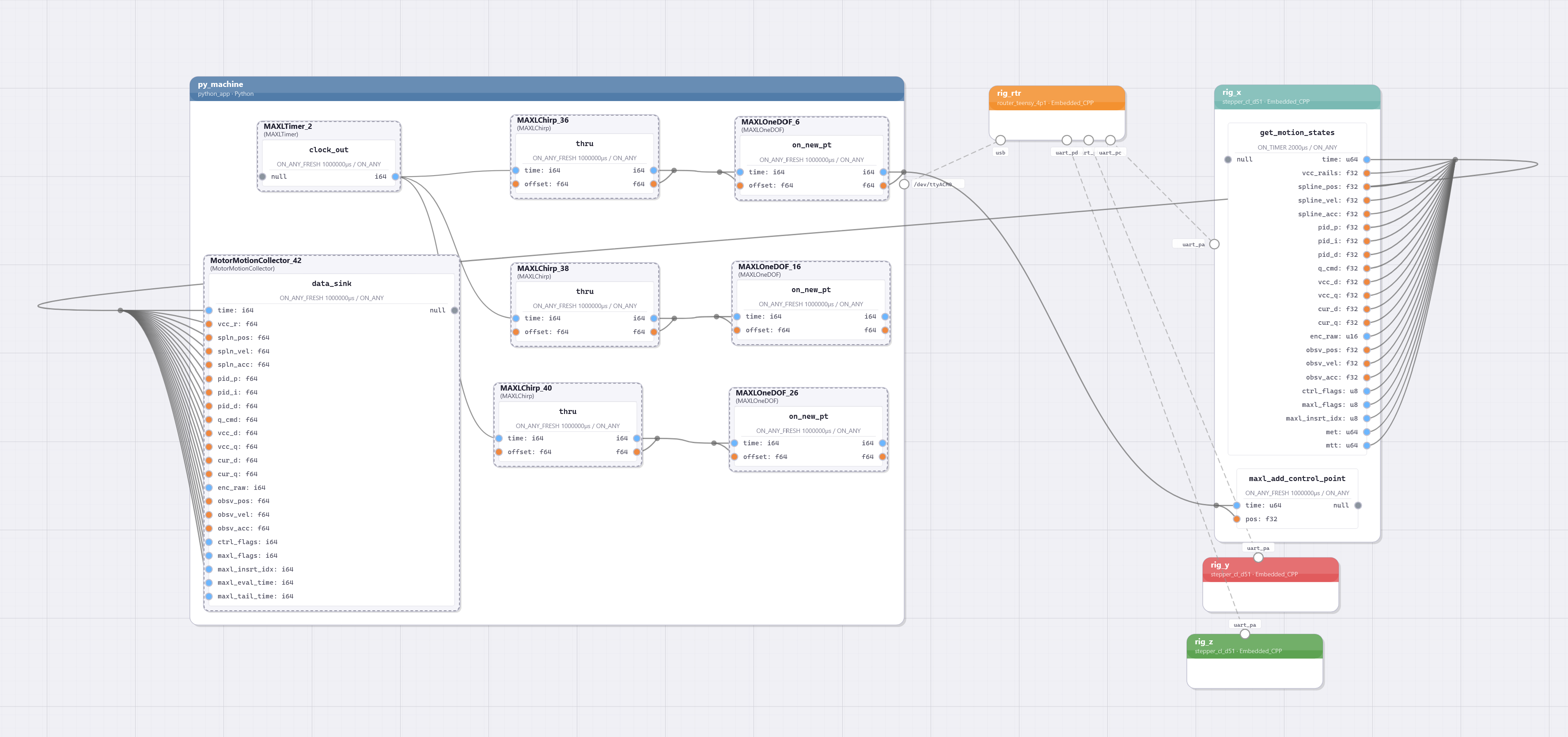
We use MAXL and PIPES to connect a Chirp block (3.3.3.3) to the axes that we are interested in fitting.

Figure 5.5: The PIPES / MAXL layout of a chirp test. The system is configured to instantiage *chirp* generators in front of each axis. These are used to drive the axes-under-test, and time-series data is collected from the motor (right) into a dataset collector (left).

Chirp parameters are configured manually, using desired displacements and a range of frequencies to cover.
Data is generated and saved.

The data from this test is useful first to tune a motor (or motors’) PID gains, which I do iteratively. This is a somewhat involved process, because improvements to gains allow us to drive the system at higher chirp frequencies - so during this process I am heuristically learning about the systems’ overall limits. However, it is a well understood process so I will not elaborate, except to note that 5.8.5 discusses how this could be automated in the future.

Even with data from poorly tuned gains, we can update our models. The only free parameters in the kinematic models are the damping terms. As in the motor models, I setup a function that estimates the motor current using the motion states (acceleration and velocity) for each axis under test, and a loss that compares that estimate to measurements from the dataset. This is the same system of equations as in Equation 5.4 (which applies to the system figured above 5.5) or in Equation 5.5 when we are sampling data from the CoreXY-based machine. Parameters that are not being fit, but are required for these estimates, are loaded from the dataset (which includes them when it loads machine definitions).

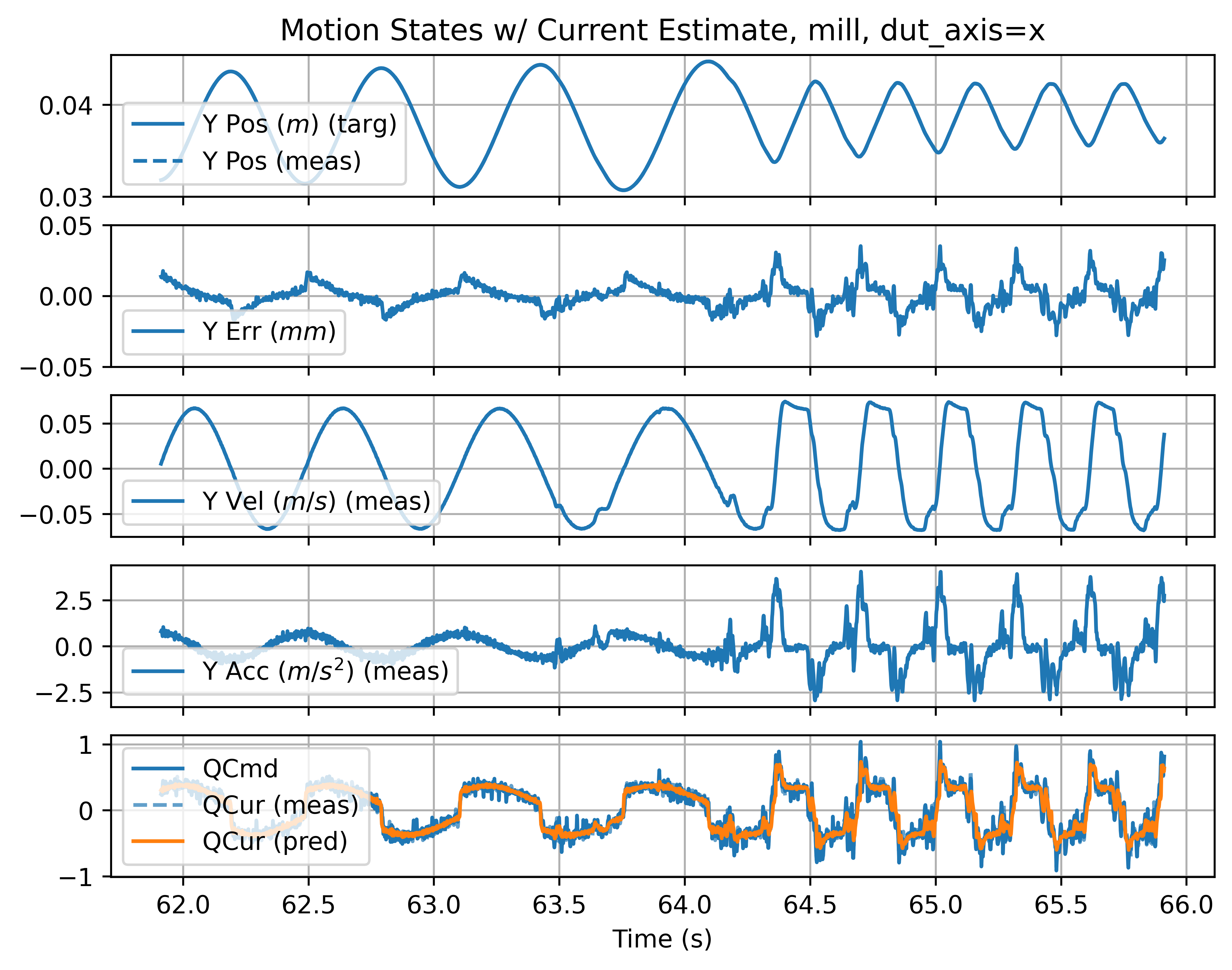
Fits can be visually verified by comparing their current estimates to measurements across time series data, as shown below.

Time-series data from a test trajectory through a CNC milling machine’s x axis, using measurements (in blue) to produce model-estimated motor currents (orange).

5.6 Optimization Based Motion Planning

With models for our machines, we can move on to planning velocities with optimization. As stated, the goal here is to choose velocities for our machine, as it travels along a target trajectory, such that those velocities are maximized without violating our actuator constraints. In this section I describe the motion control component of the solver, in Section 6.9, I describe how it can be extended to include process dynamics.

5.6.1 Optimization Formulation

I reviewed Model predictive controllers (MPCs) in Section 5.2.2. To re-orient, their basic task is to look over some horizon of control (tyipcally a fixed length time horizon) and optimize variables over that horizon such that a cost function is minimized. Calculating the cost function involves simulating the system with the chosen variables, and calculating the performance of the resulting outcome. In the case of velocity planners, the optimum outcome is normally to go fast - i.e. most velocity planners are time-optimal velocity planners.

This formulation is similar to a direct transcription method described above, but different in two key ways. The first is that the solver picks velocities in space; I take input trajectories and break them up into very many, very small line segments, a column vector of velocities in space $V(s)$. Then, rather than choosing control inputs at each step as well as those velocities, we work backwards to calculate the control inputs that would be required to achieve those velocities, and compare those to actuator limits in our cost function: violating limits is much more expensive than going slowly.

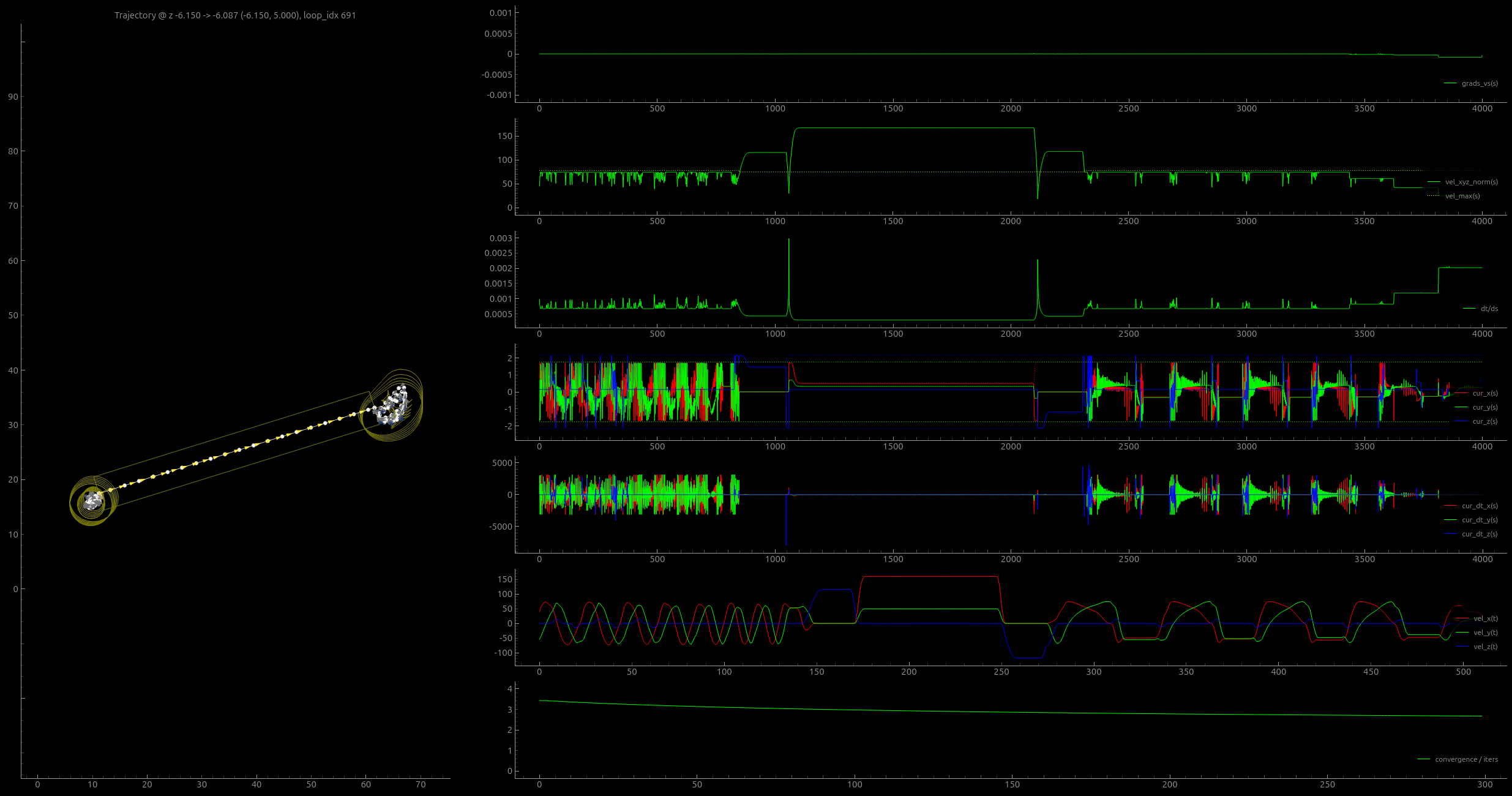
Otherwise, the solver is similar to other MPCs: the overview of the algorithm is here:

The solver is fed a spatial trajectory, which is a series of positions, each of which is a fixed displacement apart along the original (unsegmented) trajectory, I will call this $P(s)$.
We optimize over a fixed number of iterations:
1. The solver chooses $V(s)$ for each point (updated from the prior step, or initially set to some small velocity), a velocity along the trajectory.
2. We calculate the accelerations required (per axis of motion) to make the step between each velocity, $\vec{a}_{req}(s)$. We also get a series of time intervals in this step, $\Delta t(s)$
3. We calculate the actuator currents required $\vec{I}_{req}(s)$ for this $\vec{a}_{req}(s),$ in combination with the cartesian velocity at each point $\vec{v}(s),$ which our models require (for damping terms and current limits). Using $\vec{I}_{req}(s)$ and $\Delta t(s),$ we take a numerical difference to get $\vec{\frac{dI}{dt}}_{req}(s)$
4. We calculate the maximum achievable actuator currents $\vec{I}_{min,max}(s)$ at each of these $\vec{v}(s)$
5. We evaluate the solution in a cost function, large cost is added for $V(s)$ where $\vec{I}_{req}(s)$ are outside of $\vec{I}_{min,max}(s),$ small cost is added for the total time taken to travel through the trajectory.
6. The gradient of the cost with respect to $V(s)$ is computed, and an optimizer generates updates for $V(s)$ such that the cost will be minimized in the next cycle.
$V(s)$ are interpolated along $P(s)$ to produce a sequence of control points at fixed time intervals $P(t),$ a fixed length in time of which are transmitted to motors through MAXL / PIPES, call this $P_{out}(t)$
Segments of the trajectory that fall within $P_{out}(t)$ are removed from the head, and new segments are added at the tail. Previously iterated $V(s)$ are rolled back, such that the solver can continue improving these during the next cycle.
This is repeated until the input trajectory is exhausted.

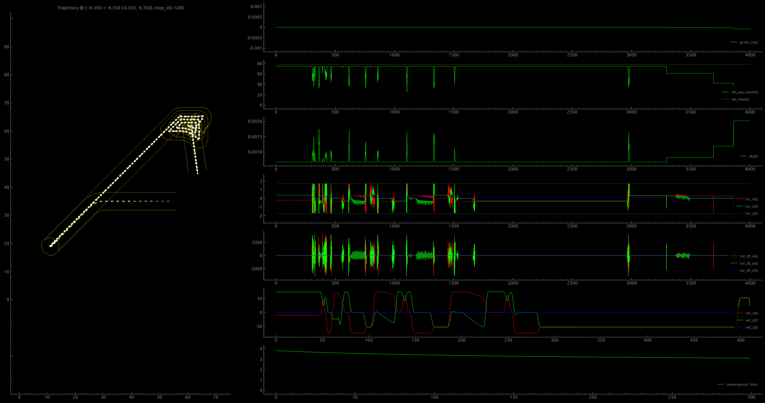
I show samples of the solver’s visualizer in two figures below, and the following subsections below describe each of the steps above in some more detail.

A frame from the solver’s output visualizer, which can run in realtime along with the machine. This is from a an “adaptive” CNC machining path. The trajectory is shown in 2D in the left side of the frame, and spatial-series data is on the right hand side, i.e. $V(s)$ is second from the top, with corresponding $\Delta t(s)$ in the third plot. Fourth and fifth are $\vec{I}_{req}(s)$ and $\vec{\frac{dI}{dt}}_{req}(s)$. The sixth plot contains *time*-series velocities for each axis. Finally, the top and bottom plot are related to the solver itself: top shows the gradient of $V(s)$ with respect to the cost function, and the bottom plot shows convergence over solver iterations.

Another frame from the same solver run, now in a section of the path that features a 2D pocket machining path.

5.6.1.1 Calculating Required Accelerations from Velocities

The chosen set of $V(s)$ are velocities along the trajectory.
This is combined with unit vectors from the trajectory to make a $\vec{v}_i, \vec{v}_f$ for each linear segment.
Now we can use the kinematic equations, one of which gets time for this step: $\Delta t = d / \frac{1}{2}(\vec{v}_i + \vec{v}_f)$ (where $d$ is the spatial step size, a solver parameter).
It is important that $\Delta t$ is positive and above some minimum and maximum size. Occasional numerical issues can cause this to happen, so we use soft_clamp to assert that is within a low- and high-band, which are also solver parameters.
The second kinematic equation in use here calculates the required acceleration for the step: $\vec{a}_{req} = (\vec{v}_f - \vec{v}_i) / \Delta t$

5.6.1.2 From Tool Tip Velocities to Actuator Currents

For this step, we use the same model as I described in Section 5.3.2. That transforms accelerations and velocities of the machine’s tool tip (in cartesian space) to currents required by our actuators:

\[ \vec{I}_{req} = f(\vec{a}_{req}, \vec{v}_{req}) \]

This step uses machine parameters that have been loaded in the solver’s configuration: kinematic functions (authored as python functions), along with damping and mass paramters. In the CNC machine, damping parameters are applied to the cartesian system alone (since the transform is $1:1$), and in the printer system, they are applied to the cartesian system as well as to the actuator states.

5.6.1.3 Minimum and Maximum Current Calculation

The cost function compares currents that would be required to actuate the proposed $V(s)$ to currents that are possible in the same states $(\vec{a}, \vec{v})$. In this context, we have actuator parameters to denote, which I map to the motor models from Section 5.3.1 in the table below.

Value	Motor Model Symbol	Solver Symbol	Solver Name
Applied voltage	$V_a$	$a_V$	Actuator voltages (supply)
Back-EMF constant	$K_e$	$a_{ke}$	Actuator $ke$
Stator impedance	$Z$	$a_Z$	Actuator impedances
Not mentioned	n/a	$a_{I,lim}$	Actuator driver current limit

The actuator voltages and driver current limit are important: these are both values that can saturate for reasons that are not described by the models themselves: maximum applied voltage is defined by the power supply’s output, and current is limited by the driver’s power electronics. Saturations are one of the most common sources of nonlinearity in real systems, this is no different. To apply these saturations without causing gradients in the solver to vanish, I use $\tanh$ to clip the values. This also leads overall more conservative use of actuators than a simple linear clip would do, and in the future the solver could be improved using a saturation function that is sharper in the transitions.

\[ \begin{aligned} a_Z &= \sqrt{a_R^2 + (a_L \cdot a_{\omega_e})^2} \\ a_{V,max} &= \tanh \left( \frac{(a_V - a_{ke}a_{\omega_e})}{a_V} \right) \cdot a_V \\ a_{I,max} &= \tanh \left( \frac{a_{V,max} / a_Z}{a_{I,lim}} \right) \cdot a_{I,lim} \\ \end{aligned} \tag{5.6}\]

The function that computes a maximum actuator current $a_{I,max}$ is also applied with negative-signed voltages to produce lower bounds for current deployment, $a_{I,min}$.

We calculate the maximum change in current $\frac{dI}{dt}$ for any step using an approximation where the maximum is the motor’s supply voltage divided by their inductances:

\[ \frac{dI}{dt}_{max} = \frac{a_V}{a_L} \tag{5.7}\]

This is technically only true when the motor is at a standstill. Looking back to our motor models 5.3.1 shows a $V_p,$ which is the voltage that can actually be applied across the stator windings. It decreases with speed: $V_p = V_a - k_e\omega_m$ where $V_a$ is the actuator voltage $(a_V)$ above. This subtlety should probably be added to the solver in the future.

5.6.1.4 The Cost Function

The cost of the solution is the sum of actuator limits violations (which prevents the solver from doing so) plus the total time to traverse the horizon (which encourages it to go fast).

The cost function needs to be smooth in order for the solver’s gradient descent algorithm to work properly. To calculate violations of constraints, I use a function that applies softmax to violations, which is modified such that it can also be tuned to normalize errors (using a scalar that is in the expected range of those values, a solver parameter), and to have a variable sized blending zone (which smooths the function). Those functions are in -#lst-solver-soft-min-max below.

Listing 5.4: Soft functions for calculating constraint violations.

def soft_err_over(val, max_val, blend_width=1.0, norm=1.0):
    """
    err for overage / out-of-bounds positive \
    blend_width = size of softplus blend zone \
    norm = expected max_val to norm errors such that 2x max = 1.0 \
    """
    hardness = 5.0 / blend_width 
    scalar = 1.0 / norm 
    omax = val - max_val
    omax_soft = (jax.nn.softplus(omax * hardness) / hardness) * scalar  

    return omax_soft 

def soft_err_over_under(val, min_val, max_val, blend_width=1.0, norm=1.0):
    """
    err for value over/under min/max \
    blend_width = size of softplus blend zone \
    norm = expected max_val to norm errors such that 2x max = 1.0 \
    """
    hardness = 5.0 / blend_width
    scalar = 1.0 / norm 

    umin = -(- min_val + val)
    omax = - max_val + val 

    umin_soft = (jax.nn.softplus(umin * hardness) / hardness) * scalar
    omax_soft = (jax.nn.softplus(omax * hardness) / hardness) * scalar

    return umin_soft, omax_soft

I mentioned in the introduction that even when we develop optimization-based control, we are likely to want to retain some heuristics-based knobs for our systems (1.3, no. 5). For motion control, I do this by encoding scalars into target trajectories that set bounds for actuator current and $\frac{dI}{dt}$ deployment, i.e. the amount of actuator effort that the solver should target. These are applied in the cost function, where $\frac{dI}{dt}_{max}, a_{I,max}$ are simply multiplied by these scalars (which are in $0, 1.0$). In Section 6.8.2.1, I discuss how these scalars are set as part of the 3D printing workflow.

5.6.1.5 Updating the Solution

The solver is structurally organized around the cost function, which returns the cost for the solver’s current $V(s),$ given a target trajectory and initial states along that trajectory. The cost function is wrapped in JAX’s value_and_grad function, which returns the cost value (to plot and debug) and the gradient. The gradient is passed to JAX’s implementatin of the adam solver (Kingma and Ba 2015), which generates updates for $V(s)$. Those are applied using Optax, and the solver iterations are all wrapped in a jit-compiled function.

Listing 5.5: The outer loop of the solver, where the cost function’s gradients are used to generate updates for the solution.

optimizer = optax.adam(params_solver_rate)
cost_func_wrapped = jax.value_and_grad(cost_func) 

@ jax.jit 
def outer_loop(params, params_i, traj_bndl):
    # params = V(s), 
    # params_i = V(s=0), the initial state from the prior solution 
    def step(carry, _):
        _params, opt_state = carry 
        cost, grads = cost_func_wrapped(_params, params_i, traj_bndl)
        updates, opt_state = optimizer.update(grads, opt_state) 
        _params = optax.apply_updates(_params, updates) 
        return (_params, opt_state), (cost, grads)  

    # jax.lax.scan causes the entire cycle of optimizer iterations
    # to be compiled together, i.e. this is just a jaxlike loop
    (params_f, opt_state_f), (costs_f, grads_f) = jax.lax.scan(
        step,
        (params, optimizer.init(params)),
        xs=None,
        length=params_solver_steps
    )

    return params_f, costs_f, grads_f

5.6.1.6 From Space to Time

In the final step, we need to deliver part of the solution to hardware, and roll the trajectory horizon into the future. The hardware operates on a fixed time interval, whereas the solver’s internal states are all defined in fixed spatial steps.

So, the first task in this step is to transform $V(s)$ along the trajectory $P(s)$ into some $P(t)$. This is done by interpolating a new time series along a function that describes the time at each spatial step $t(s),$ which is just a cumulative sum of the $\Delta t$ mentioned above.

Segments that are within the transmitted time window are removed from the head of the trajectory, and new points are added at the tail. The solved points are transmitted to an interface class that is connected to hardware (or running as a simulation), as I describe below.

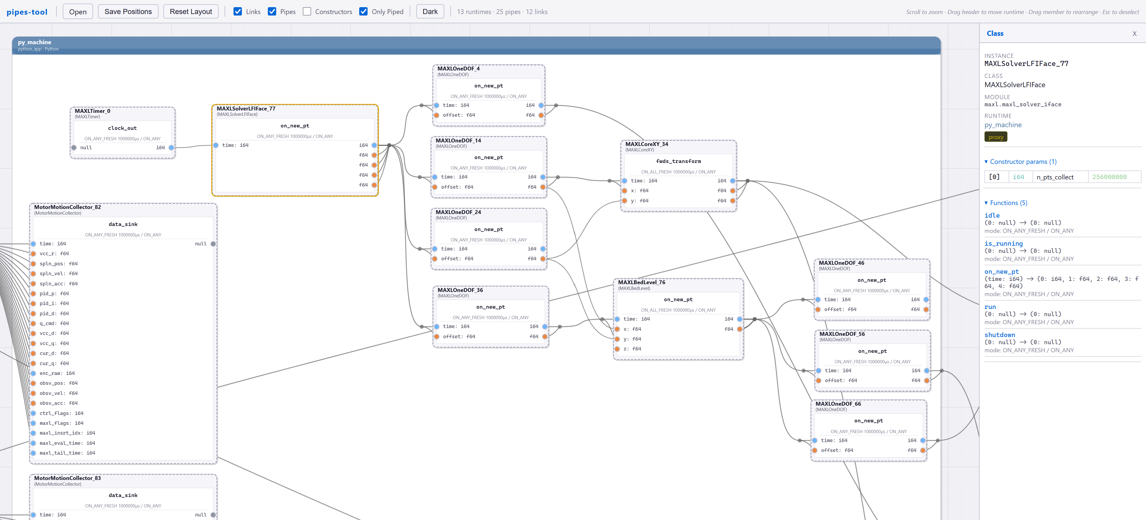
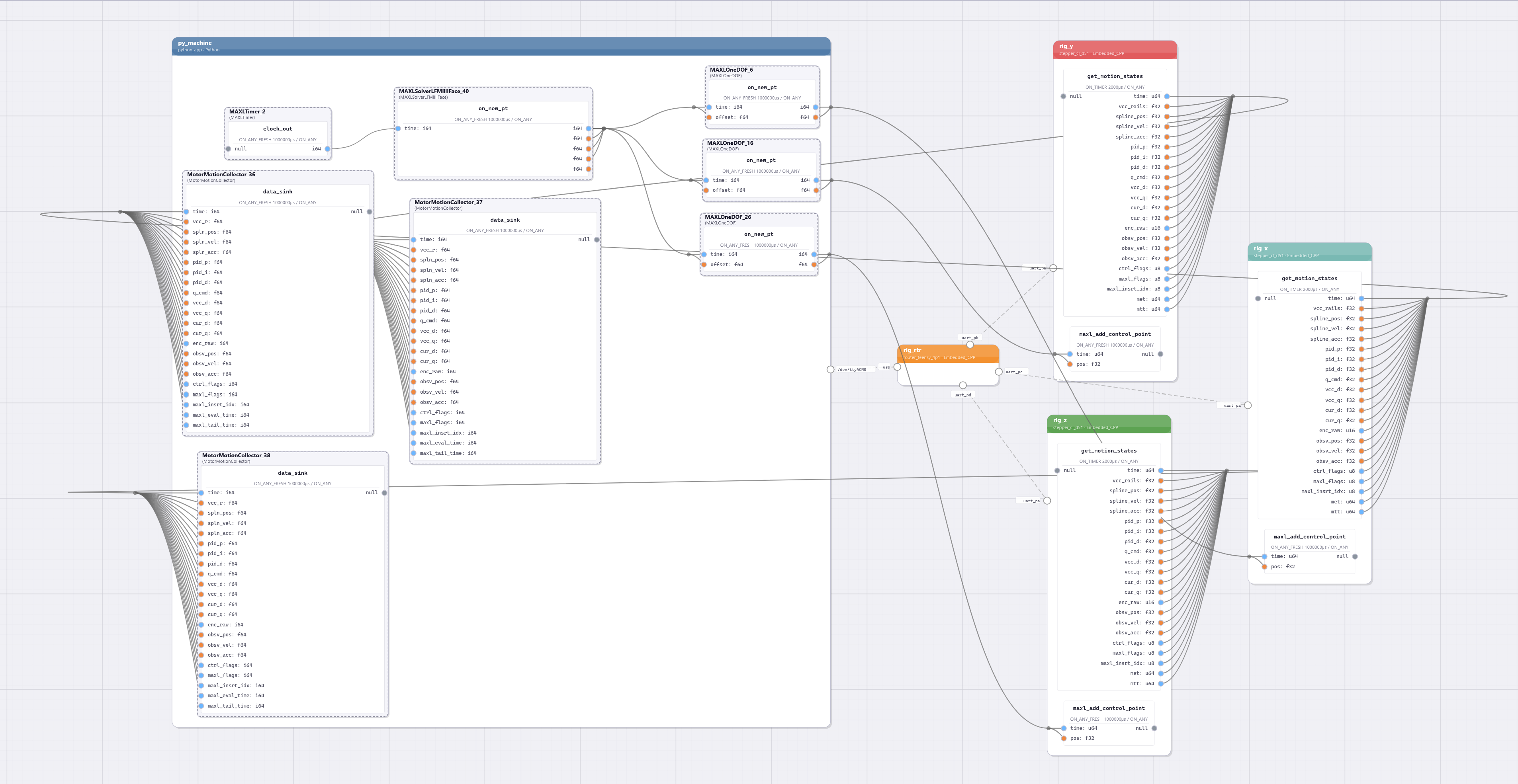
5.6.2 Pipelining the Solver

Some more detail on how the solver is integrated into the machine, and how it cycles through trajectories.

Complete run files are loaded into the solver when it launches. It is connected to a MAXL / PIPES system via an interface class, which itself is connected to the solver via an os-level socket in python. This prevents the solver from locking the rest of the system up while it is generating new solutions.

Figure 5.6: The FrankenPrusa’s (6.4.2) solver (highlighted in orange) makes up one component in that machine’s PIPES graph 3.2. This view is centered on the python components in the machine, hardware is represented out of frame.

The CNC milling machine from Chapter 7, configured to use the solver for motion planning. Motors are rendered in the right side of the frame.

The interface class also saves stores solver outputs directly, for later evaluation i.e. in 6.11.2 (and in results from this section).

It is important to note that while the solver runs in realtime, it does not receive realtime feedback from hardware; the solver is a feed-forward planning step. It updates at $10Hz$ only; spatial horizions are quite long ($500mm$ in the printer, and $300mm$ for the milling machine). I call it feedback-based primarily because the models that it uses are developed on the hardware to which is connected. I discuss this in some more detail in 5.8.6.

5.7 Results

5.7.1 Trapezoids vs Model-Based Control

The solver allows us to use more of our motion systems’ dynamic range than trapezoidal solvers because they use models that describe motion limits in the full range of acceleration and velocity states. Trapezoidal solvers used fixed values: a maximum acceleration and a maximum velocity (per axis of cartesian motion).

In Section 7.3.1, I show that we can use models to select these parameters for trapezoidal solvers. An example of one such selection is below. The shaded area marks the space where the trapezoidal solver can operate. However, the real boundary (marked by $550N,$ a force margin) encloses a larger area, especially in the left-hand side of the plot.

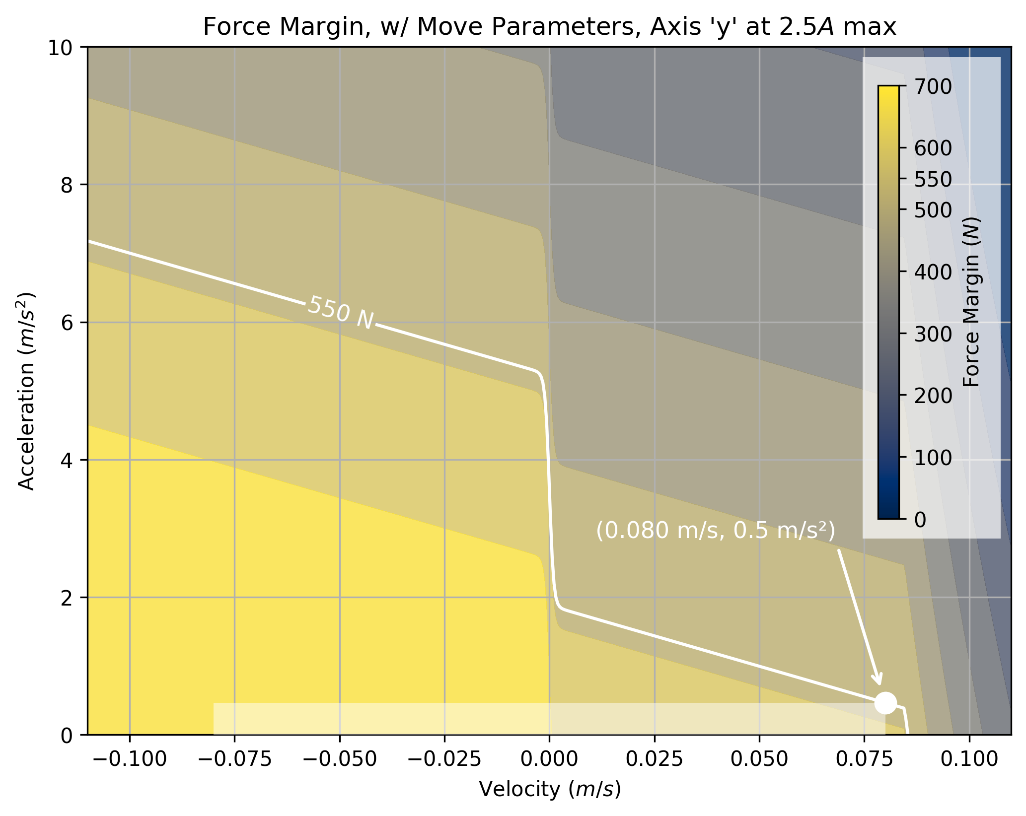
The system modelled in these images has a large damping offset. When we are accelerating against the current velocity, that damping can actually work in our favour. This dynamic is not exploited by trapezoidal solvers. We can see this clearly if we look at motion states traversed during a test part by a trapezoid planner using these parameters.

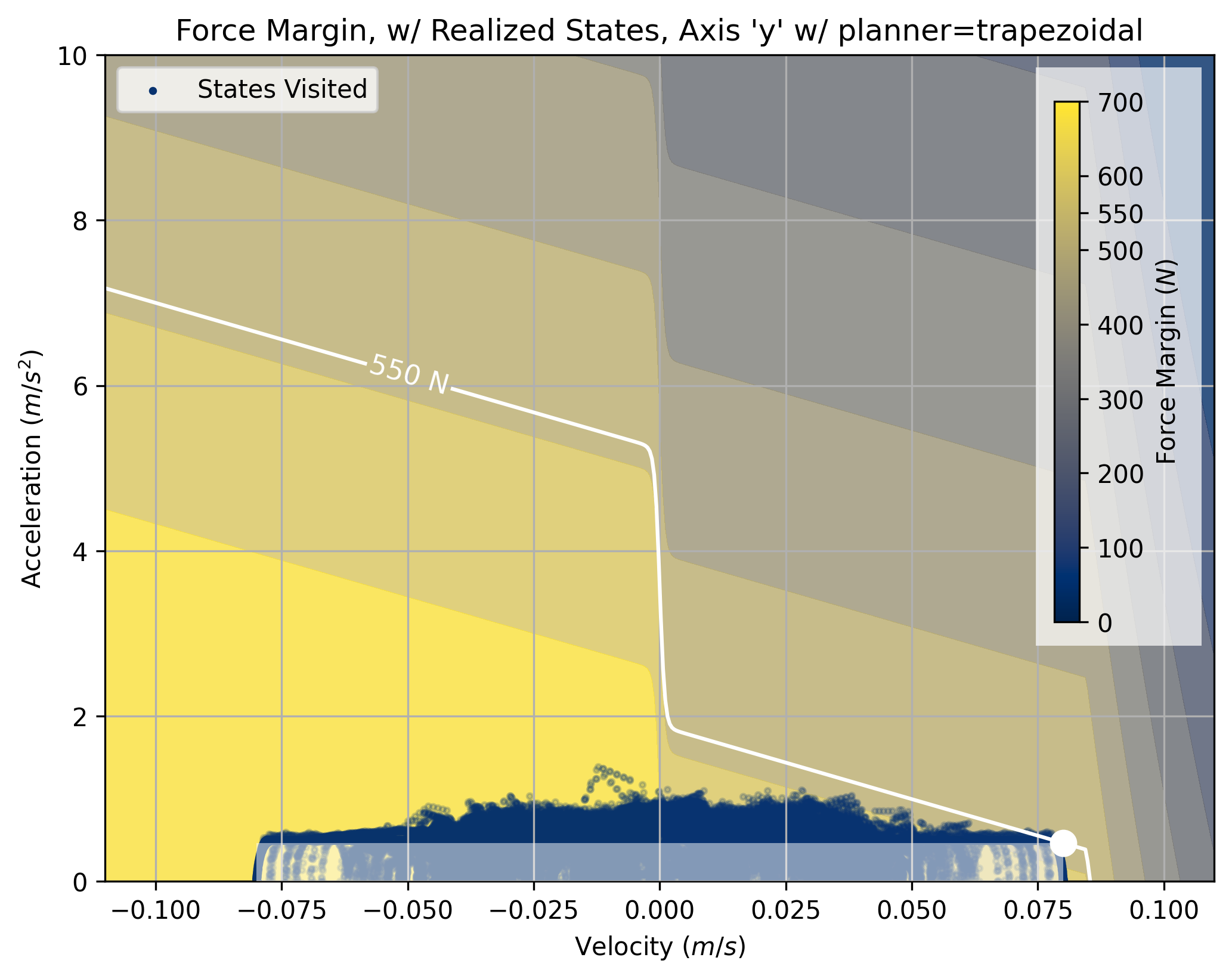
States visited by a trapezoidal planner when it was configured to operate within the shaded rectangle.

The boundary is still violated somewhat by the trapezoidal solver. This is an artefact from the junction deviation step, which causes the machine to execute accelerations that are actually somewhat larger than the specified maximum. See 5.2.1 for more detail.

If we run the same target trajectory with the optimizer, we can see that more states are used - again, especially in the left-hand side of the plot.

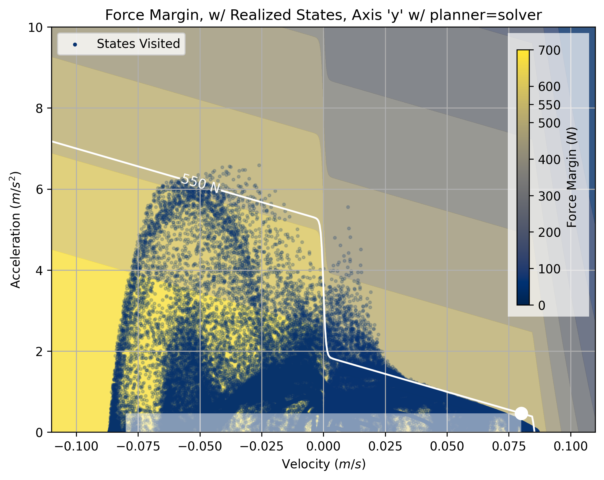
States visited by the optimizer as it plans velocities for the same path as in the figure above. Here, the solver is meant to be able to operate everwhere under the force margin.

There is some lossiness here, too - near the origin we can see a cloud of points that exceed the specified force margin. I believe that this is an artefact of the solver’s own lossy cornering step (5.6.1.1). I discuss how a more direct use of splines in the solver could reduce these errors in Section 5.8.3.3. However, this shows that model-based motion planners have potential to greatly improve machine performance.

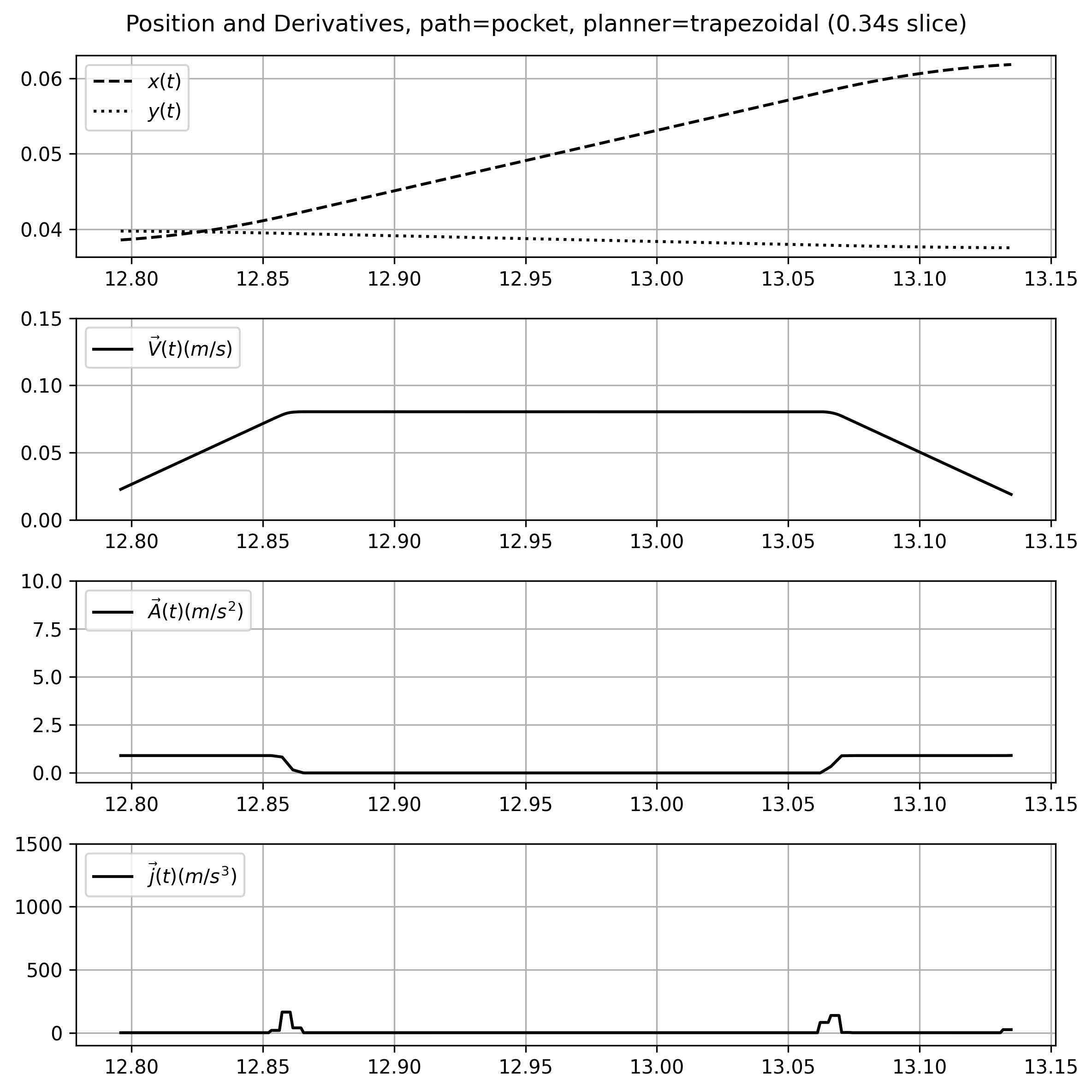
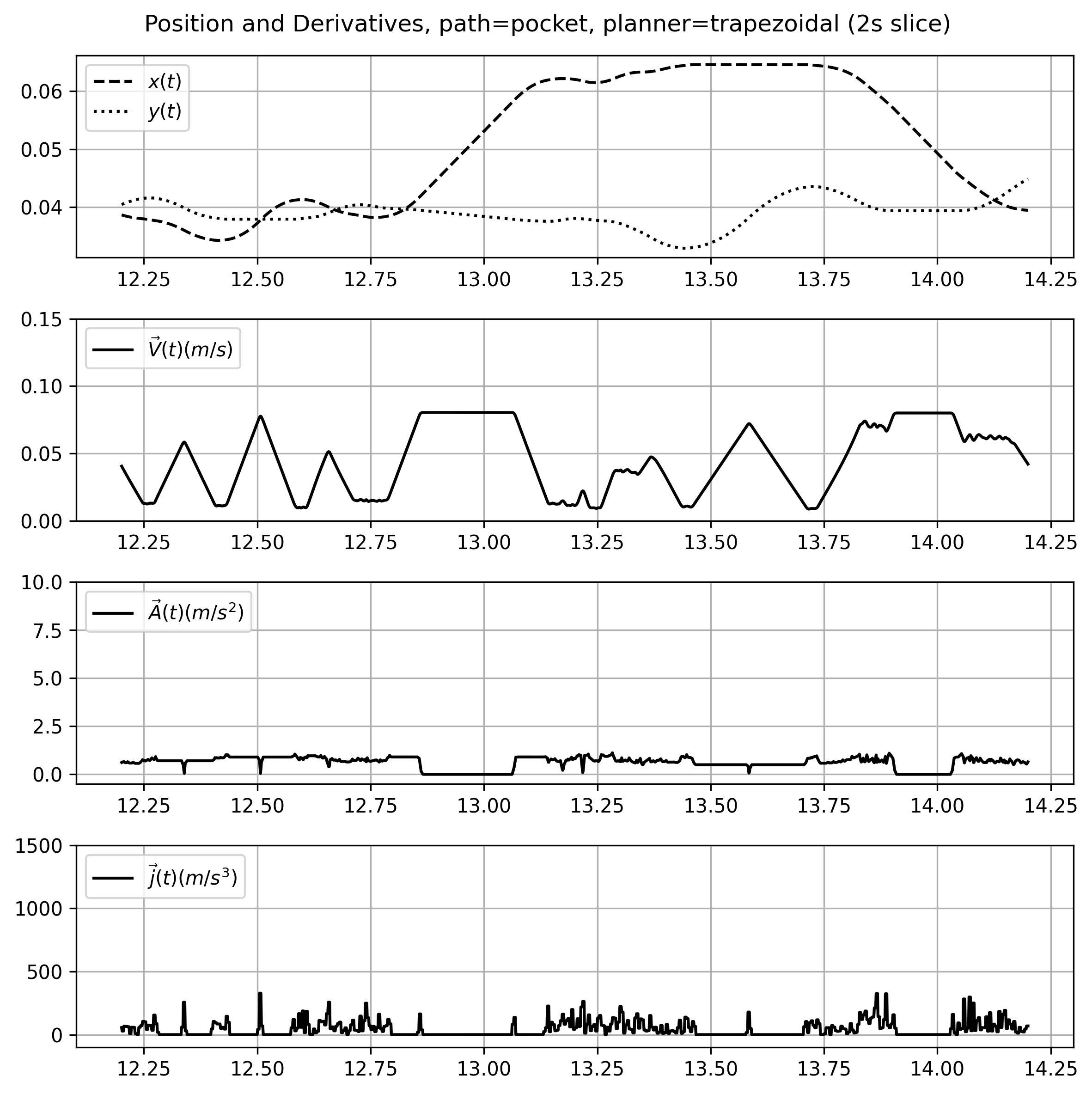
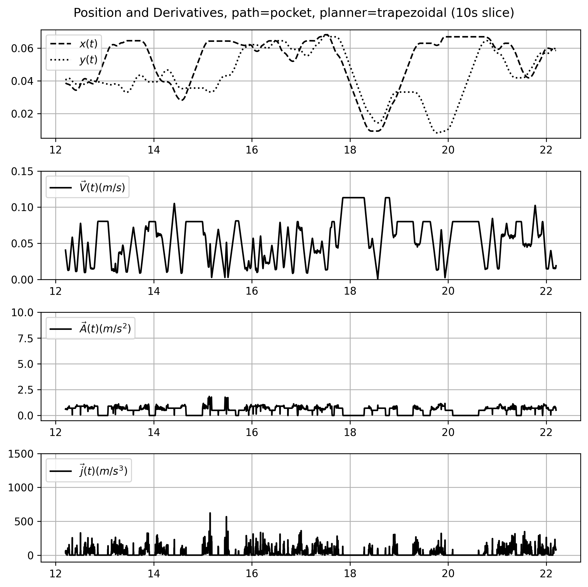
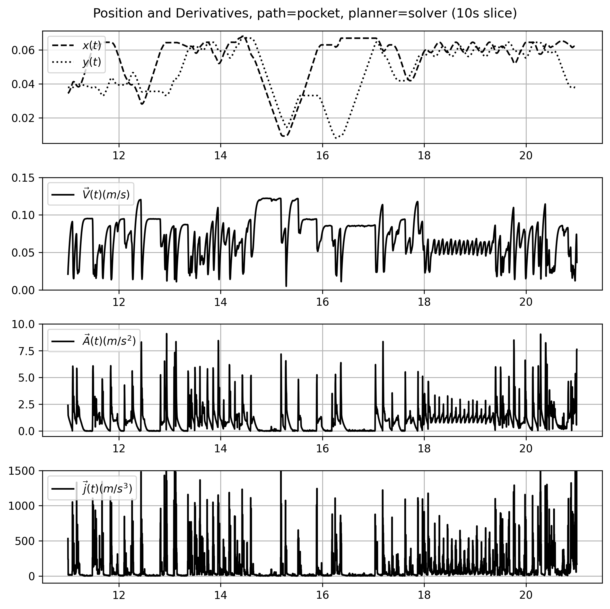
The difference between the solver and trapezoid planners is evident also when we look at the velocity-time plots that they generate, a comparison of which is below.

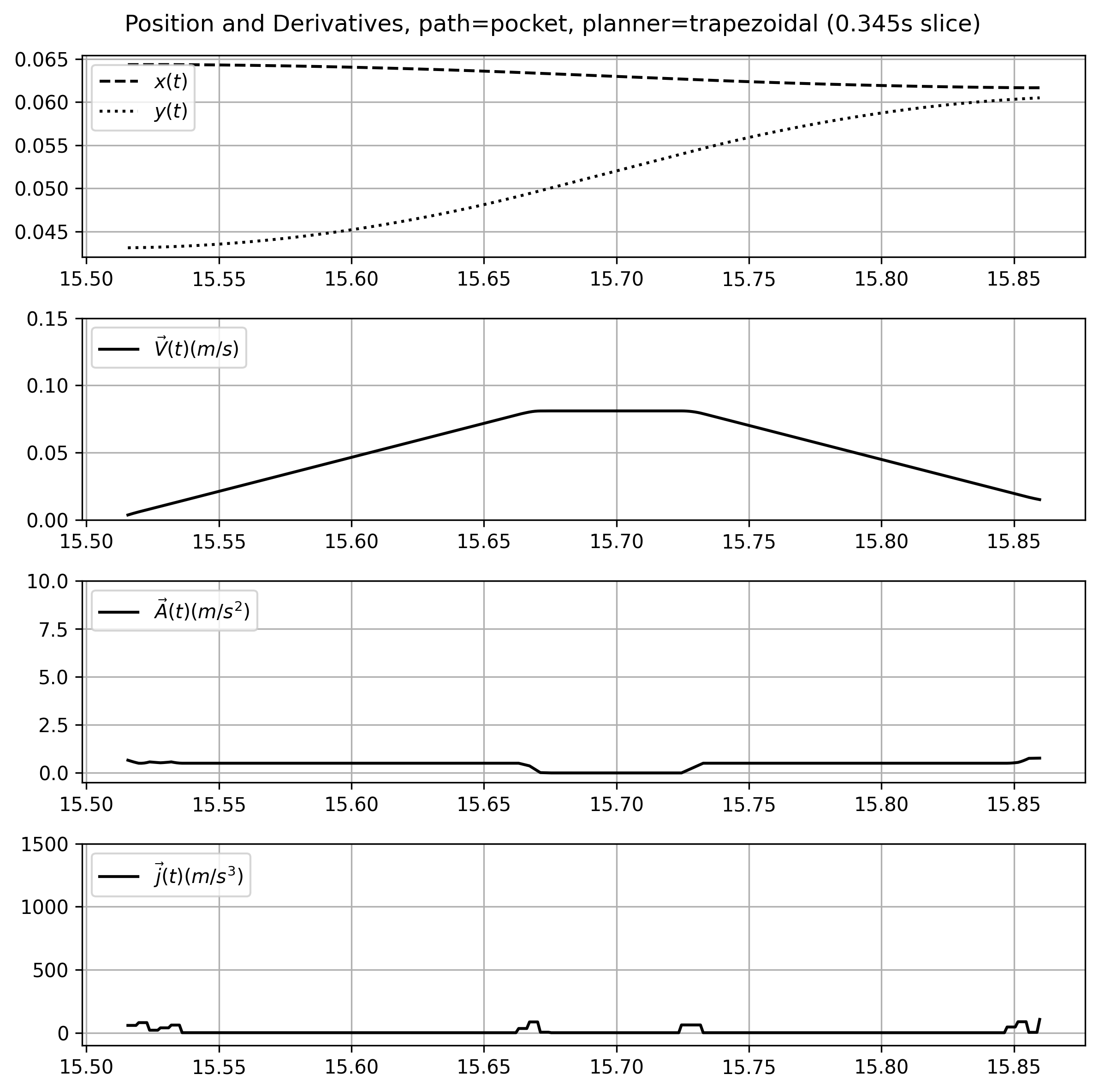
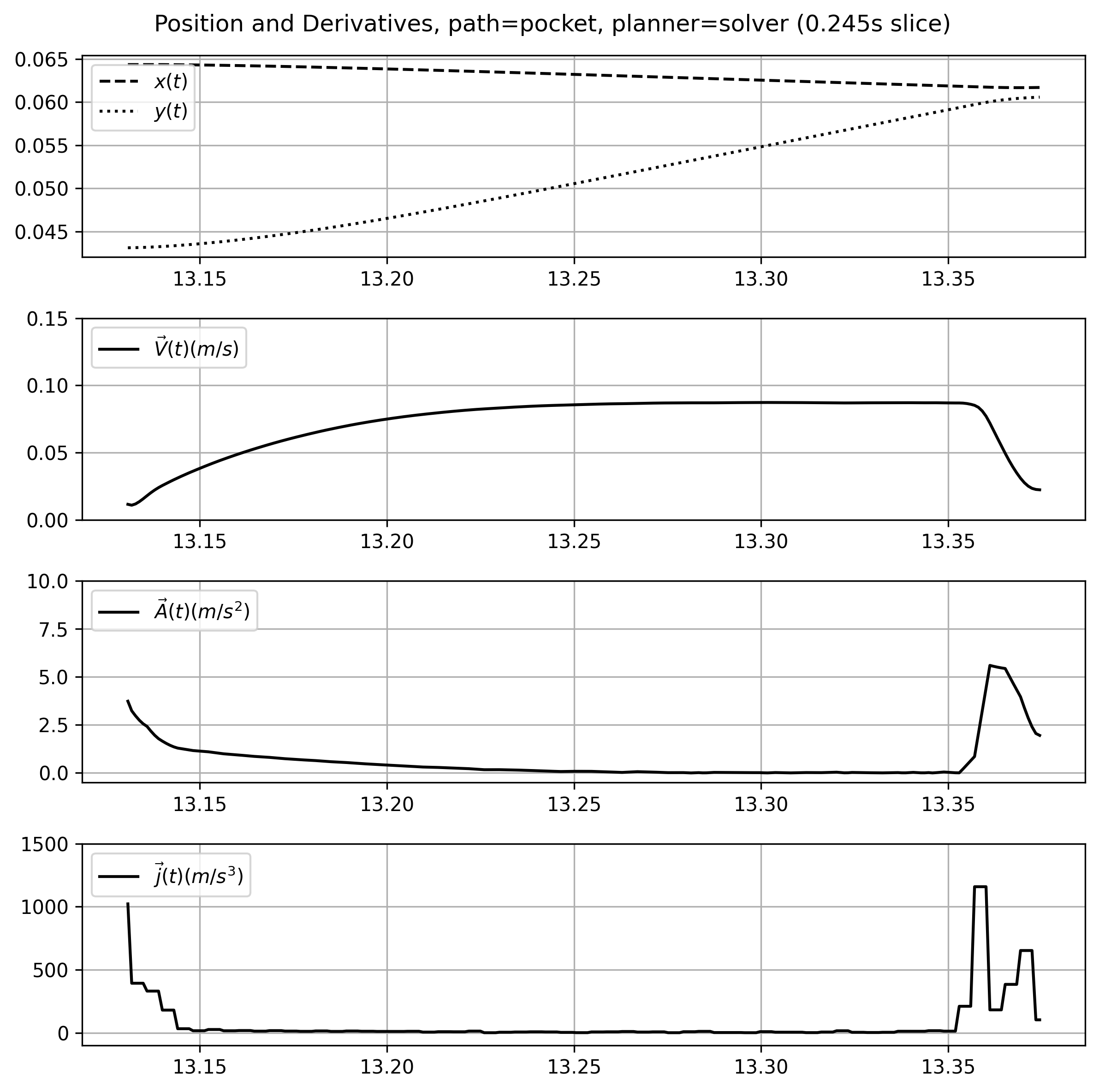
Figure 5.7: Position, velocity, acceleration and jerk time-series data from a trapezoid solver (left) and our planner (right).

We can see that the solver exploits the system’s damping dynamics: the front half of the speed curve (where it is working against friction) is much shallower than the tail, where it is working with friction. These plots are taken over the same trajectory segment: the solver also traverses it in less time $(0.245s \ vs \ 0.345s)$

We can also see that the solver uses more acceleration more regularely, and that acceleration is variable with respect to the system speed: a result of damping and motor dynamics together.

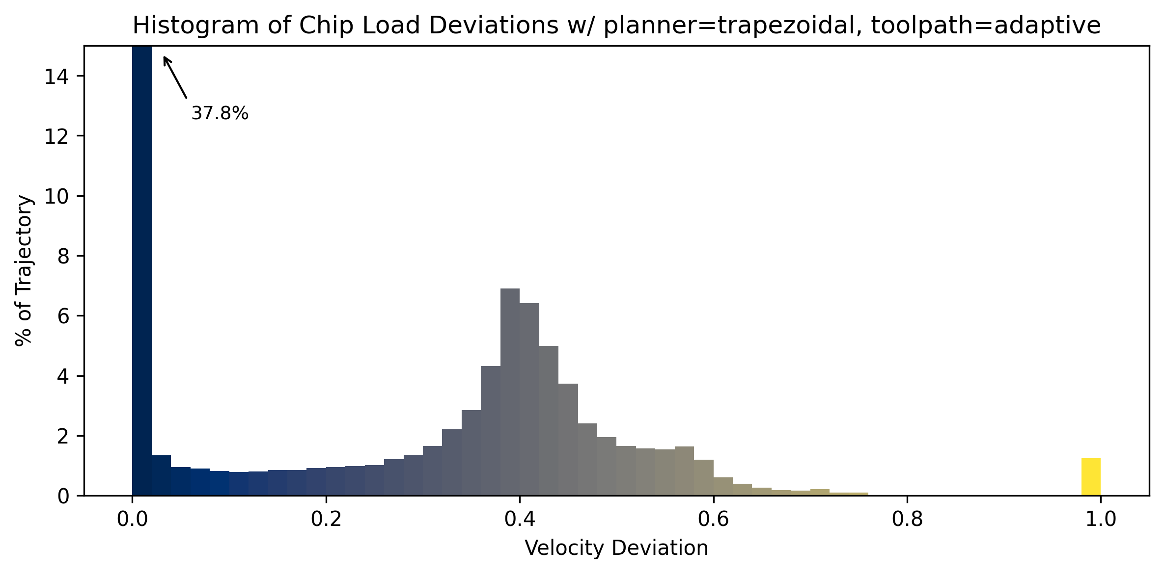
Figure 5.8: Position, velocity, acceleration and jerk time-series data from a trapezoid solver (left) and our planner (right).

In CNC machining, maintaining feedrates such that they match users’s cut parameters is of critical importance - when machine speeds decrease, chip sizes changes as well. When chips become too small, the cutting tool begins to rub instead of cut, which can cause chip welding. I discuss this in Section 7.2.1.

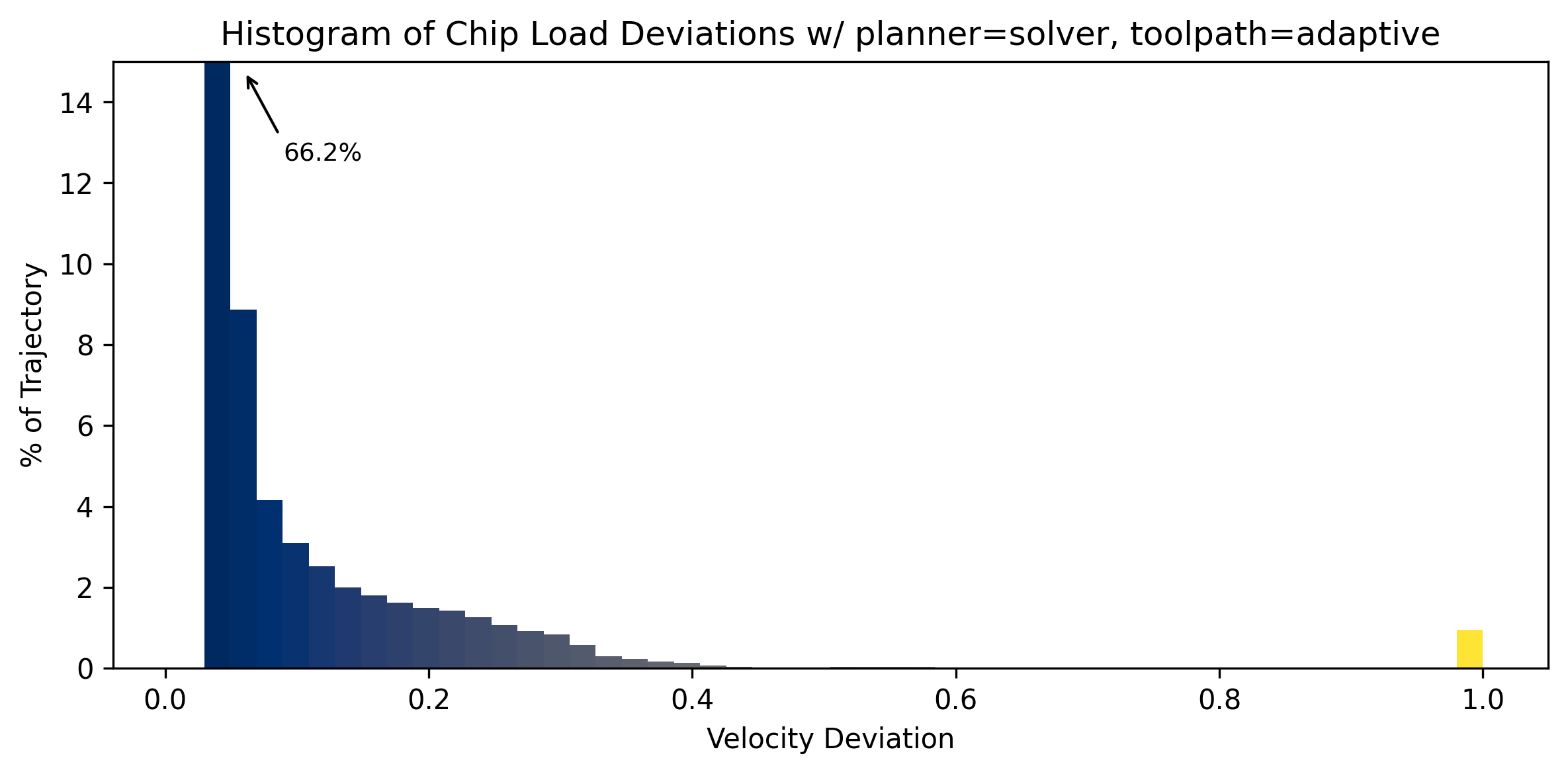
Because I developed a method to pick parameters for a trapezoidal planner using motion models and did so for a milling machine in Section 7.5.2, I was able to compare the optimizer’s performance against a trapezoidal planner where we know that the trapezoidal planners’ motion parameters are not simply under-tuned. For this comparison, I use the trapezoid planner that I developed for MAXL 3.3.3.4. MAXL / PIPES also lets us swap between the two planners without making any other changes to the system.

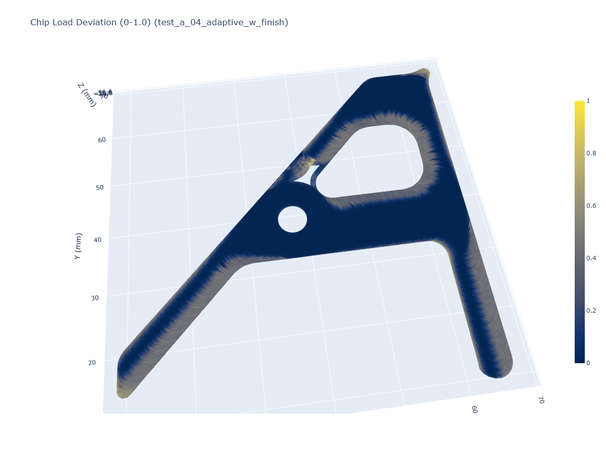
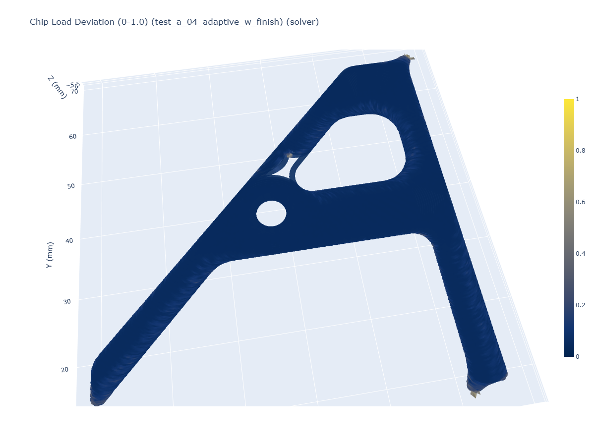
Figure 5.9: 3D heat map of deviations from target velocity from the same target trajectory, using a trapezoid planner (left) and the solver from this section (right).

We can see that velocity deviations are greatly reduced when the solver is used. This is observable also in histograms that show the distribution of deviations over the course of the entire trajectory.

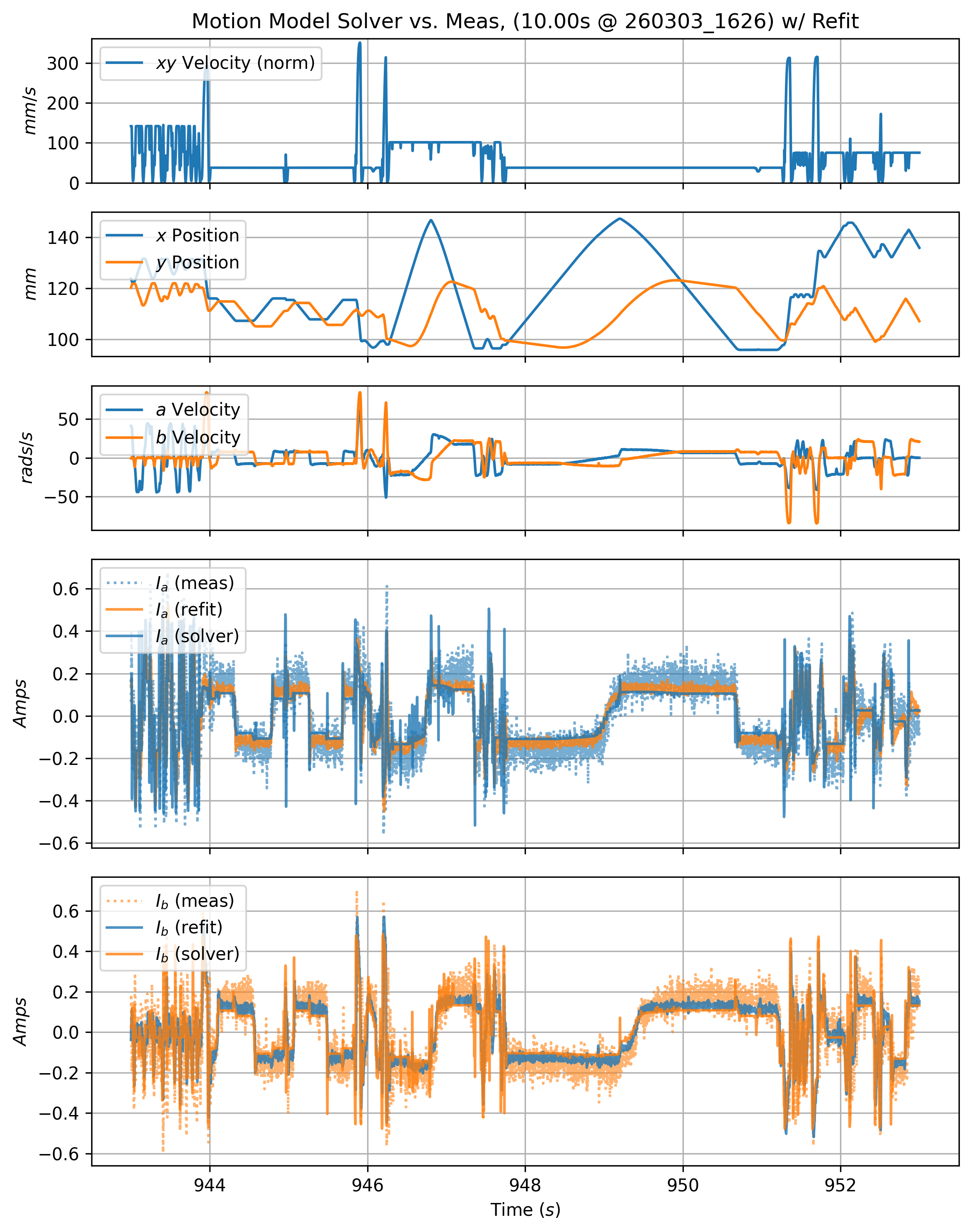
Figure 5.10: Distribution of deviations from target velocity from the same target trajectory, using a trapezoid planner (left) and the solver from this section (right).

5.7.2 Model-Fit Quality

In Section 6.10.1, results from each part include an error metric on motion model fits. This metric measures the average deviation of the solver’s motor current estimates from measured motor states. Those are calculated from time-series like those shown below, which renders a twelve second slice of motion data from one of the prints. In it, we can see predicted motor currents (solid lines) vs. measured currents (dotted lines with some transparency).

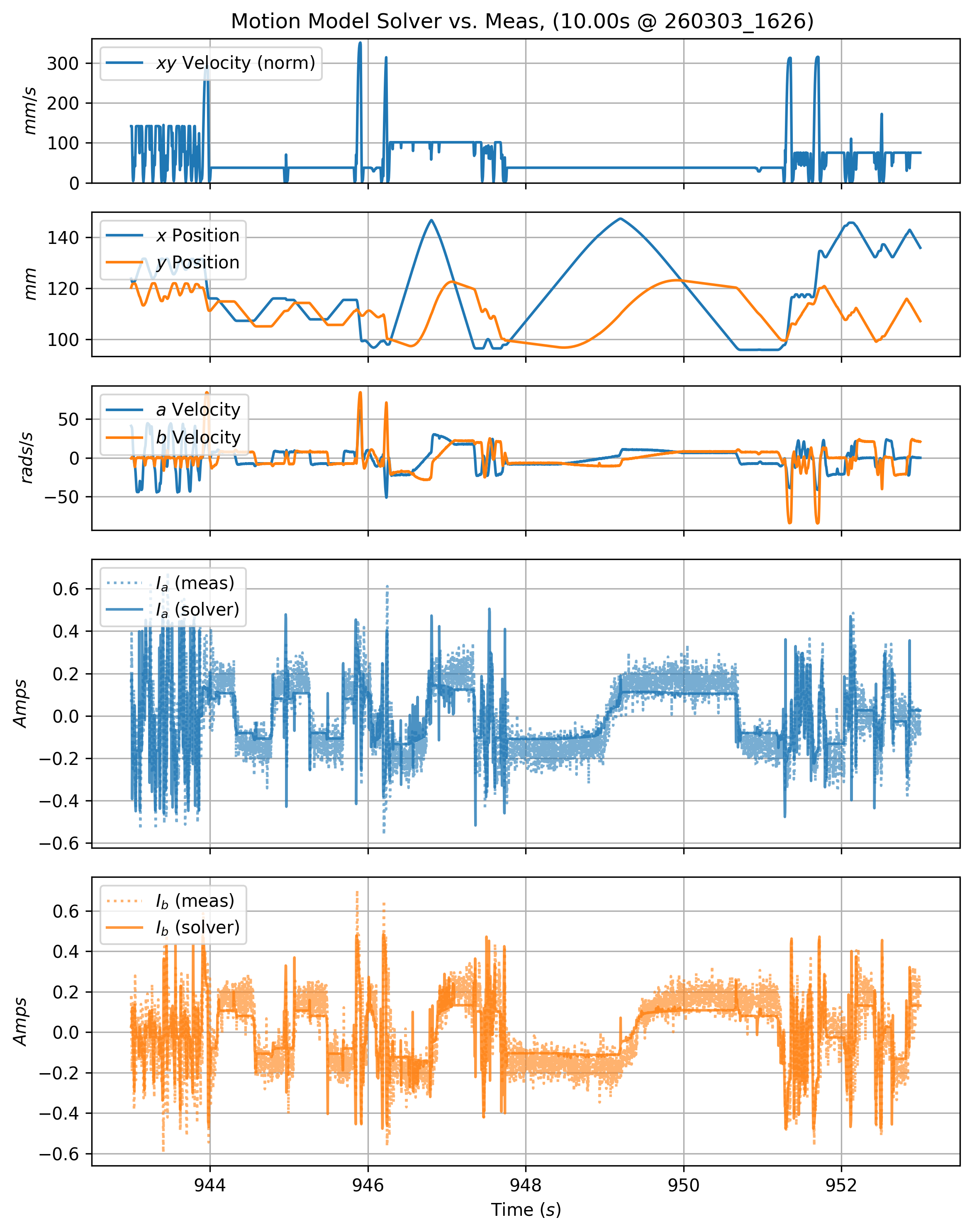
Figure 5.11: Time series comparison the system’s motion measurements (dotted lines) with the solver’s predictions (solid lines), for a subset of a print job.

On average, the printer models deviated from measurements by $0.175 A,$ which is considerable. These errors emerge partially due to noise emitted by the motor’s PID controllers, which are tuned to be quite stiff. However, it is clear that the model fit is not excellent. The fits are initially performed on chirp data (per 5.5.2), but real-world machine control spans more states than those generated in the chirp test.

I also modified the printer between the chirp tests and operation, tightening its belts. This increases damping, which I forgot to account for by running new tests. However, noticing this leads us well into the next section here.

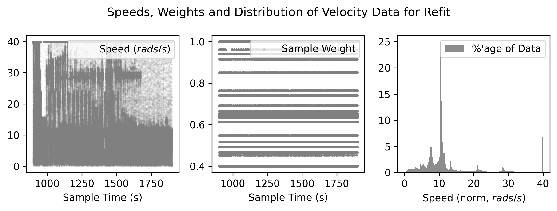
5.7.3 Continous Improvement of Models

Because our hardware is also our testing equipment, we can re-fit motion models on data that we collect during regular operation, i.e. the 3D plot below shows current estimate errors in 3D from the FFF printer.

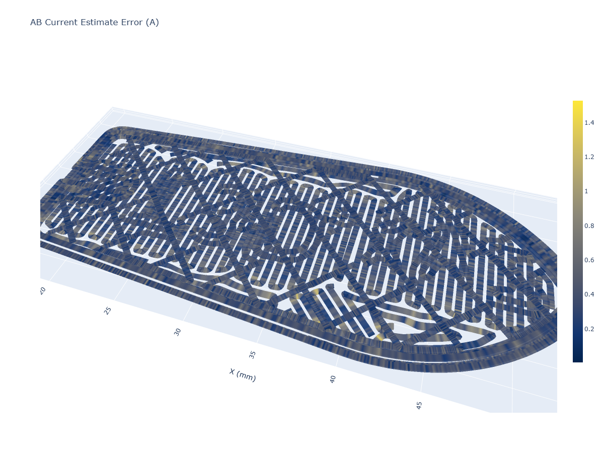
Motion Current Error with initial Inertia and Damping Estimates

Refits are done with weights, which help the fitting routine to oversample in regions of machine velocity that are over-represented.

Figure 5.12: Time series data from the printer, as above, but now including improved current estimates, calculated using model updates.

5.8 Discussion

5.8.1 Machining with Trapezoidal vs. Model-Based Velocity Planning

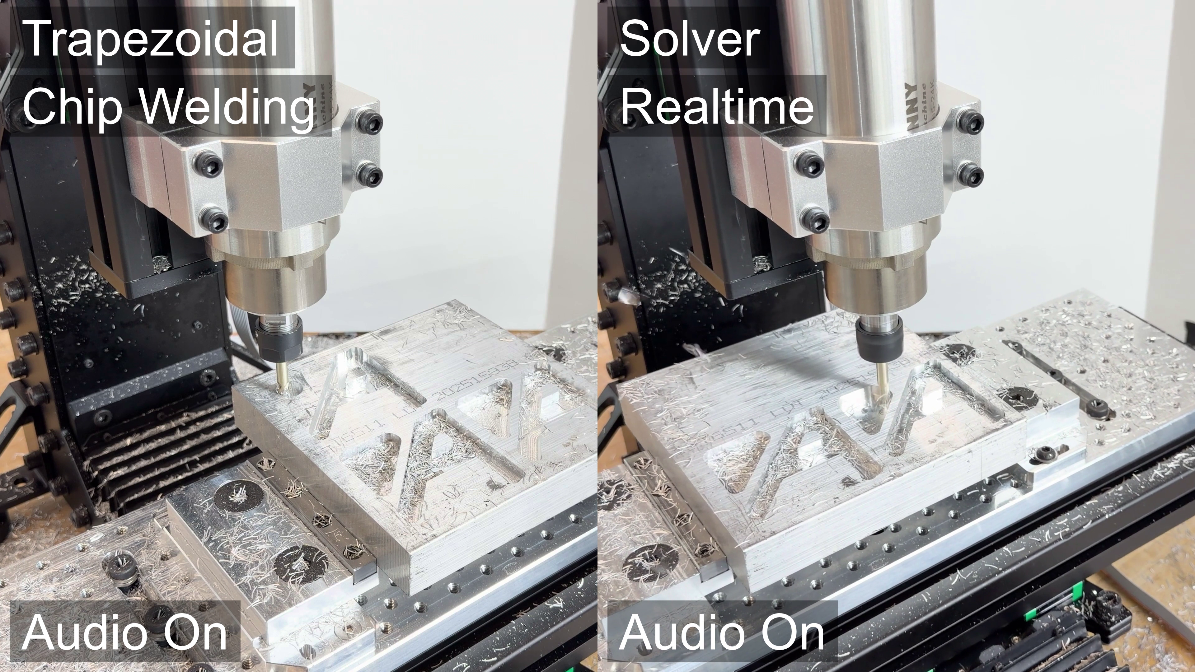
I discussed a one-to-one comparison of a trapezoid planner to the solver in Section 5.7.1. I was able to actually run these jobs on hardware. In these comparison runs (see video here), I saw two things of note.

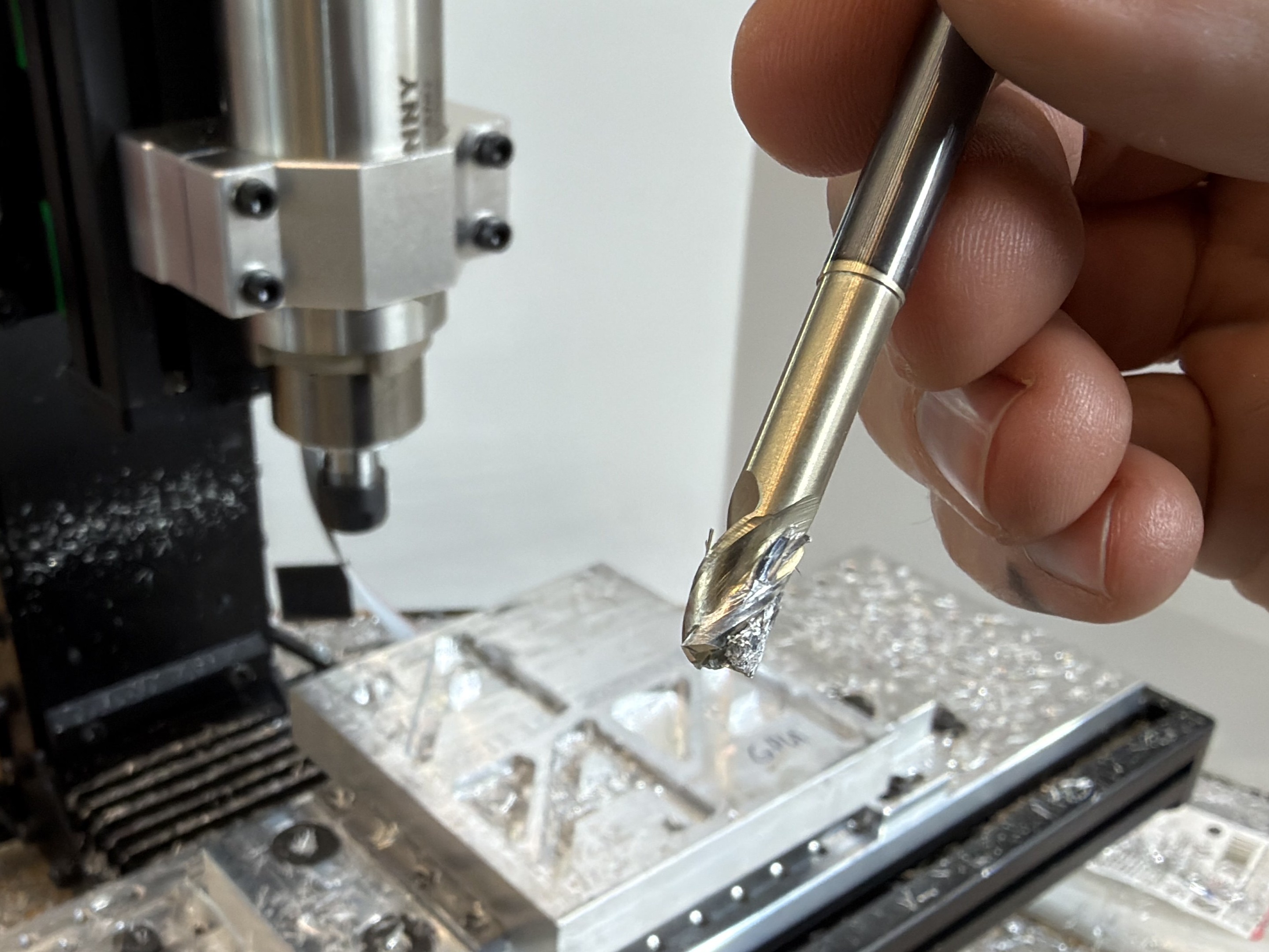
First, it becomes clear that the solver is faster overall after the first few cuts. This is audible as well, there is a subtle difference to the sound that the machine makes as it enters a cut: with the solver, the cutting sound is more consistent (perhaps indicating uniform process parameters through the cut), whereas there is an audible ramp in tone in the trapezoid solver.

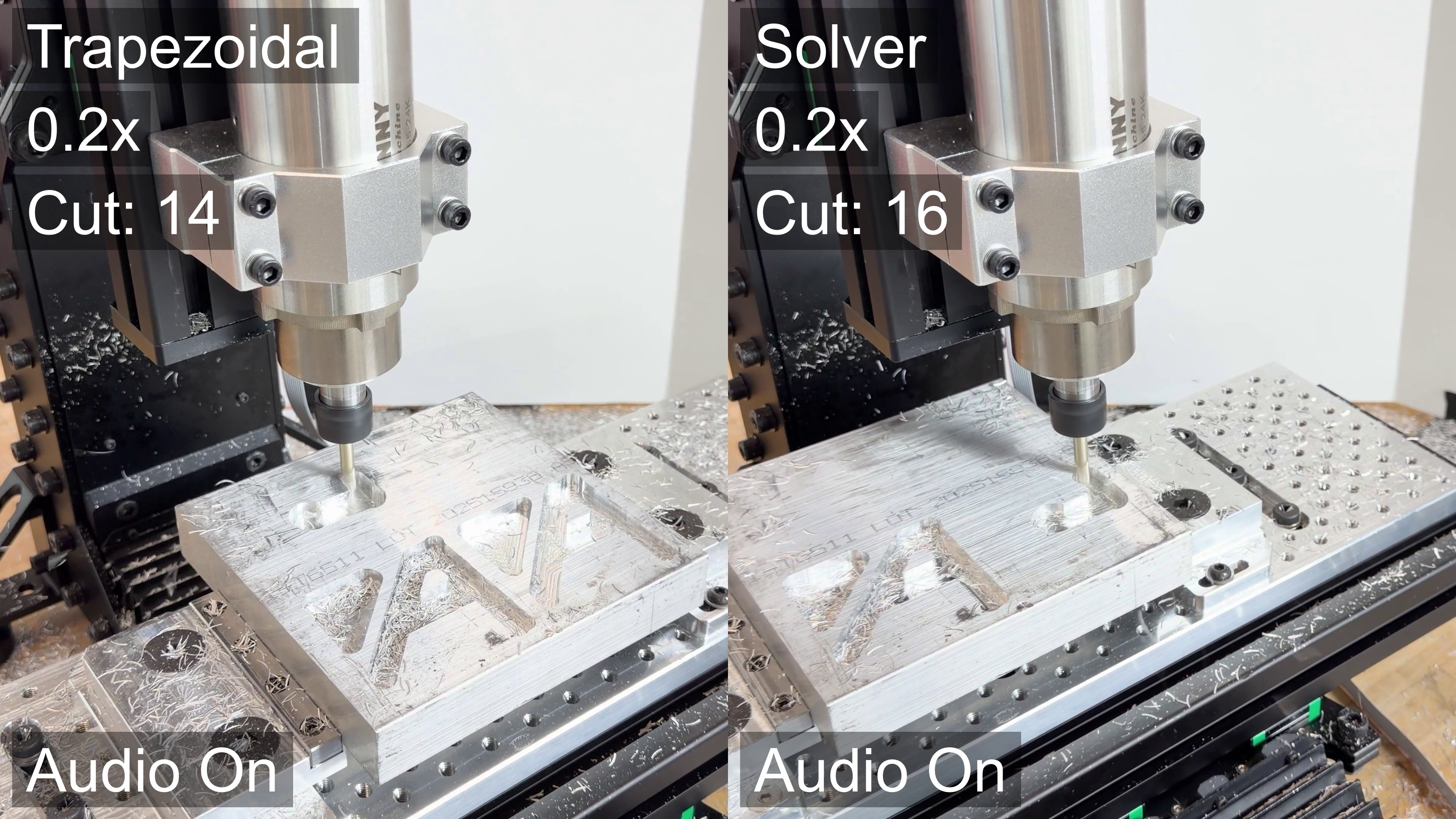
The premise is that maintaining chip load reduces the likelihood of chip welding, and (while this doesn’t constitute a rigorous evaluation), I could not get the trapezoidally-controlled toolpath to finish the cut without welding the endmill.

This shows how variable machining can be: the toolpath is the same as I had run a number of times previously, when I ran the experiments in Section 7.5.3. I tried the trapezoidal path a total of three times, each with a fresh endmill. The solver-controller run worked on the first attempt, and I tested it between one failed trapezoidal path and another. My guess is that in this case there was less time between jobs. In my prior runs of this part, I took a few minutes between each cut to adjust parameters in the toolpath. This time I was simply running paths one after another. The stock was warm to the touch during these experiments - perhaps the chip welding was more likely because of this increased temperature, however slight. This would also indicate that the toolpath parameters that I found in 7.5.3 were quite close to the limits.

Chip welding on the endmill used in this experiment.

5.8.2 Notes on Motor Models

promised to discuss torque/speed trade-off in sec-cnc, should also discuss how even two motors of the same make, model can have variable parameters, as mentioned in the final discussion.

5.8.3 Notes on the Solver

5.8.3.1 Piling In to the Cost Function

(about s-curves) tying processes in to these planners can be cumbersome, as they use incomplete models and “think linearly” - i.e. we can’t arbitrarily add constraints - as I will show in the next chapter, our solver architecture allows us to add process control physics w/o explicitly re-authoring the motion control component to accomodate. the soln’ presented here is flexible in that we can basically throw whatever tf we want into the solvers’ cost function, and we lean on GPU / AutoDiff magic to make it work…

5.8.3.2 About Performance and Hyperparameters

Without process control, performance (on a modern GPU) is not limiting. Once cost function becomes heavy (and we add i.e. time dependence in the printer solver), things do get tight. It was common that I had to re-tune solver parameters (optimization rate, steps, size of the problem) to get it solving properly, and in time.
Performance favours larger chunks solved at once, due to hot-start… on the GPU, where bandwidth into and out of the GPU kernel (and between python and that backend) is tight, we want larger horizons at larger ticks - which does not lend itself towards true real-time feedback.

5.8.3.3 The Spline Disconnect

While our solver works in $v(s),$ motors evaluate basis splines (from Section 3.3). Although the lossiness of this handoff is minimal , it really seems as though we aught to be able to solve the spline outputs directly, rather than doing this whole dance in Section 5.6.2.
This would be especially valuable in lower performance networks where spline intervals may be large: we should be able to add spline deviation to the cost function, to maintain some epsilon here.
In particular, this causes issues w/ the step in Section 5.6.1.1. Splines should give us these $A$ directly…

5.8.3.4 About GPUs for Motion Control

… “so you’re telling me I need a GPU to control my machine?”

I know, it seems insane. While this controller is measurably better than other solutions, it runs expensive computing hardware. For example, during the development of this thesis I used an RTX 4070 GPU ($700) to run machines whose BOM costs were between $200 and $800 each. Of course this trade-off might not seem as insane were we talking about half-million dollar milling machines.

Two notes on that: first, this is the advantage of being a researcher: we can occasionally make insanely strange economic choices and then simply make statement like (second note:) compute hardware for “AI” (i.e. GPUs) is currently one of the most over-invested fields in the world. At the time of writing, NVIDIA’s (who makes GPUs) valuation is something like 7% of the USA’s GDP. Smells like a bubble to me, but when this one pops the cost of this computing hardware will be a tenth of what it is currently.

A third note on that is that the optimizers developed here do not need big GPUs, just baby ones. This application takes up only 200Mb of VRAM, for example. The oracles in the (silicon) valley would expect the level of GPU required here is likely to be available for tens-of-dollars in the near future.

5.8.4 MIA: Frequency Domain

I had assumed that motors and kinematics would explain most of the limits to overall motion performance. This turned out not to be the case: stiffness (and it’s friend, resonance) is.
I did some experiments using not fast fourier transforms to asses and remove energy in some bands…
- don’t have the kit to assess frequency response,
- properly done it would be expressed as stiffness and damping terms,
- properly calculated it should be possible to assess spring loading for selected velocities: we did the equivalent of this in the extruder system,
- simple may be: for any given accelerating load, we can calculate spring displacement under that load, prevent large $\frac{dD}{dt}$ (where $D=spring \ compression$) …

5.8.5 MIA: Computational PIDs and Motor Measurements

I did a lot of work to model motors and motion systems, and yet a critical step in this process is my hand-tuning of motor PIDS. I developed tools for this, so it wasn’t so bad, but there is lots of literature on the topic and it should be possible to have automated this, too.
This is a classic case where the controller interacts with the model: in fact we would need to model i.e. noise in the encoder, delay from the observer (and tune its gains), etc.
This dependence actually speaks to a broader miss in this thesis: we should be able to tune through multiple layers of these models… i.e. update encoder calibrations, motor models and pids, kalman gains, and motion and kinematic models all together with data collected during machine operation. In practice, teasing each of these components apart is difficult and we wind up with systems where a parameter fitting routine could either tune i.e. $k_t$ or end effector mass to fit the same data. One approach to solve this may be to collapse model terms where we can identify that they are degenerate… better normalization of data through state spaces, etc…
Final note: the implied goal of Section 5.4 is that our controller should be deployable, somewhat automatically, on many different stepper motors. Measurements of motor $R, L$ and pole pair counts are possible to do using the controller itself, rather than (in the case of $L$), a somewhat expensive LCR probe. Perhaps most difficult is estimating also the rotor inertia, as error in it’s estimation can easily slip into the motor’s $k_t$ value; although it should not slip into the value for $k_e,$ so it can perhaps be distinguished form data. Overall on topics like this, I think extending the modelling techniques used to quantify uncertainty about parameter fits is a clear next step for the work overall.

5.8.6 Open vs. Closed Loop Motion

Closed loop has many benefits… however, so does open loop - aka feed forward.
Open Loop is often used as a dirty word: but when it is done well (with models, to make really precise feed forward terms), it is wonderful. The world’s fastest systems are mostly feed forward, using loop closing essentially just as a backstop for unforseen disturbances. It has zero phase delay, etc.
In closed loop, our PIDs (or whatever is down there) introduce some phase delay. For extremely crispy motion, this is sometimes the limit. Tuning PIDs up to this limit is difficult, as they become more susceptible to instabilities.

5.9 Future Work

5.9.1 Stiffness and Resonance

Move to Future Work / Discussion ?
- discussion: ’tis missing frequency domain…
  - connect that to machining, where freq. domain critical
  - connect that to the printer, where it became obvious that the real limit to machine speed is not motor current potential (heuristics were de-tuned to the order of 1/10th available), but is actually mostly limited to belt stretch, belt vibration, and structural deformation under heavy acceleration.
models also miss externalities like shearing teeth on belts, gears etc (although these could be added to our relatively flexible cost function, as other domains to avoid)
Mechanical Resonance
- everything vibrates… exciting resonances is bad,
- using an acceleromter, we can send input chirp thru motion system in each mechanical DOF, and FFT the output to find peaks…
- difference between measured acceleration and end effector and measured at motors, thru kinematic model, is related to stiffness of system,
- current @ motors, thru model, relates to damping,

5.9.2 Generalizing Kinematics

… kinematic discovery from-scratch ? symbolic regression ? cameras ?

There is a lot that I didn’t get to on the topic of motion control. Probably the most frustrating of which is the task of more generally fitting kinematic models from motion data. The idea here would be that we could develop well known motor models, attach those to new machines, and automatically discover how they are configured vis-a-vis the machine’s transmission elements and mechanisms. This would be invaluable to machine builders because working out kinematic models is cumbersome first in getting configurations correct (motor offsets, transmission ratios), and then for refining those models: machines never go together exactly the way they are planned (no two lines are completely parallel, etc), and to achieve real precision we often need to fit kinematic models to data. For example the simple task of figuring out a machine’s exact working volume is often done with simple trial and error.

A series of plotters developed by participants in a workshop that I co-hosted at the CBA with Ilan Moyer and Leo McElroy. Participants were each experienced machine builders, but not experienced controls engineers. We were able to use MAXl to develop working kinematic models for each of these machines.

In some proposed schemes, we could develop a library of possible kinematic arrangements, attach an accelerometer to the end effector (as I have done here to work out resonances), and learn how each actuator’s acceleration corresponds to end effector motion. Backing out linear transforms is presumably as easy as filling in the matrix that relates one system to the other (see EQN (?)), but nonlinear transforms would also require that we guess the composition of the transform function and its inverse. Inprecise models like neural networks might get close in this regard, but are probably too much of a black-box to be truly suitable to the task: in machine design and control, it is invaluable to have precise definitions of our core systems.

Adding computer vision to learn kinematic models more concretely is another proposal (or hybrids of each), and my colleage Quentin Bolsee is working on this currently at the CBA. There are a littany of other data collection approaches for this task: probing known geometries (like the method outlined for bed leveling in this work) is a common one, and could be extended to correct for XY kinematics as well as in Z (as is in fact common on some 3D printers).

5.9.3 A Spec for Machine Digital Twins

One of the ideas that developed as I was working on these controllers is that of interfacing the (already software-based) controller to a “digital twin” of the whole machine. I think the most productive version of this idea is to use the digital twin as an interface between the machine designers’ understanding of their hardware’s kinematics and the controller.

FIGURE: little-guy, and printer digital twin
COMPARE: ROS Robot Description Language ?

For example we can normally take for granted that a machine designer will have a mostly complete CAD model of their output. Those CAD models are normally assembled using constraints that generate mechanisms: linear slides, rotary joints, etc - everything we need for a rigid body simulation.

A hope had been that we could develop a representation of these assemblies that could be exported from a CAD tool and plugged directly into the solver: the solver could then run and visualize the machine virtually to ensure that the designer’s idea of how the machine was going to move matched to reality. Data from motors could be used to verify and improve these alignments in all of the ways I’ve discussed previously. This representation could be as simple as a set of .stl or .step of the rigid bodies, and some .xml or .json outlining their relations to one another (joint types, etc), as well as linkages to actuators.

The goal of this tool would be to enable machine designers to quickly bring their machines to life, using a representation and interface (their CAD model) that they are already familiar with. Some such projects exist, i.e. ROBOT_XML (?), etc… yada yada - done well, the tool could also help machine designers learn about their designs’ performance before they build it, i.e. that a motor should be made more or less powerful, or a transmission element made stiffer, or that their mechanism could be improved to increase the machine’s range of motion, etc…

5.9.4 Composing Motion Systems for Automation

Another aspect that I wish I had been able to develop more completely is the idea of using graphs of functional blocks to compose motion systems. I originally spoke with Ilan Moyer about this idea some years ago, soon after I had realized that basis splines were a suitable representation for fluid motion⁴. The control points are so simple to transform (including through nonlinear transforms), since they alone are stateless: we can simply think of transforming position to position. However, we can also do transforms that change through time since they are continuously generated, i.e. applying an acceleration limit, etc.

More generally this some “flow of positions in time” that can be transformed arbitrarily, and it means that we can also i.e. record points, replay them, loop them, multiply them, add and subtract offsets, etc. This opens the door not just to better planning algorithms but to more abstract realtime control for tool-building: each transform block can be controlled by some other input: direct user controls, inputs from other motion systems, etc. Ilan came up with a lot of these ideas and has since finished some really excellent work, implementing it with a system that transforms step and direction pulses directly, rather than the more abstract basis spline.

The core principles should extend to make it possible to very quickly build automation more generally: conveyors, material handlers, etc: imagine all of the machines in a bottling plant. These are all subject to motion dynamics, but across “n dofs,” some of which are coupled but many are not. Graphs that contain motion flows and normal logic elements could be a really good framework for assembling their controllers.

References

Albus, James Sacra, Anthony J Barbera, Roger N Nagel, et al. 1980. Theory and Practice of Hierarchical Control. National Bureau of Standards Gaithersburg, MD, USA.

Ay, Muzaffer, Max Schwenzer, Sebastian Stemmler, Adrian Karl Rüppel, Dirk Abel, and Thomas Bergs. 2022. “Practical Nonlinear Model Predictive Control of a CNC Machining Center with Support Vector Machines.” In 2022 IEEE/ASME International Conference on Advanced Intelligent Mechatronics (AIM), 1625–31. IEEE. https://doi.org/10.1109/AIM52237.2022.9863354.

Bartlett, Roscoe A., Lorenz T. Biegler, Johan Backström, and Vipin Gopal. 2002. “Quadratic Programming Algorithms for Large-Scale Model Predictive Control.” Journal of Process Control 12 (7): 775–95. https://doi.org/10.1016/S0959-1524(02)00002-1.

Brunton, Steven L, and J Nathan Kutz. 2022a. “Chapter 11: Reinforcement Learning.” In Data-Driven Science and Engineering: Machine Learning, Dynamical Systems, and Control, 419–44. Cambridge, United Kingdom: Cambridge University Press.

———. 2022b. Data-Driven Science and Engineering: Machine Learning, Dynamical Systems, and Control. Cambridge, United Kingdom: Cambridge University Press.

Conroy, Phillip. 2018. “Computing Junction Deviation for Marlin Firmware.” Blog post, Kynetic CNC. http://blog.kyneticcnc.com/2018/10/computing-junction-deviation-for-marlin.html.

DeepMind. 2024. “Optax: Composable Gradient Processing and Optimization Library for JAX.” https://github.com/deepmind/optax.

Di Carlo, Jared, Patrick M Wensing, Benjamin Katz, Gerardo Bledt, and Sangbae Kim. 2018. “Dynamic Locomotion in the Mit Cheetah 3 Through Convex Model-Predictive Control.” In 2018 IEEE/RSJ International Conference on Intelligent Robots and Systems (IROS), 1–9. IEEE.

Douglas, Brian. 2012. “PID Control – A Brief Introduction.” YouTube, Control Systems Lectures. https://www.youtube.com/watch?v=UR0hOmjaHp0.

Giorgio Bort, Carlos Maximiliano, Marco Leonesio, and Paolo Bosetti. 2016. “A Model-Based Adaptive Controller for Chatter Mitigation and Productivity Enhancement in CNC Milling Machines.” Robotics and Computer-Integrated Manufacturing 40: 34–43. https://doi.org/10.1016/j.rcim.2016.01.006.

(https://electronics.stackexchange.com/users/330/jason-s), Jason S. n.d. “Understanding Motor Constants Kt and Kemf for Comparing Brushless DC Motors.” Electrical Engineering Stack Exchange. https://electronics.stackexchange.com/q/33332.

Hyun, Dong Jin, Sangok Seok, Jongwoo Lee, and Sangbae Kim. 2014. “High Speed Trot-Running: Implementation of a Hierarchical Controller Using Proprioceptive Impedance Control on the MIT Cheetah.” The International Journal of Robotics Research 33 (11): 1417–45.

Jeon, Sungeun K. 2011. “Improving Grbl: Cornering Algorithm.” Blog post, One Hoss Shay. https://onehossshay.wordpress.com/2011/09/24/improving_grbl_cornering_algorithm/.

Jeon, Sungeun K., Simen Svale Skogsrud, and Jens Geisler. 2011--2024. “Grbl: An Open Source, Embedded, High Performance g-Code Parser and CNC Milling Controller.” GitHub repository. https://github.com/gnea/grbl.

Kalman, Rudolf E. 1960. “A New Approach to Linear Filtering and Prediction Problems.” Transactions of the ASME – Journal of Basic Engineering 82 (1): 35–45. https://doi.org/10.1115/1.3662552.

Kaufmann, Elia, Leonard Bauersfeld, Antonio Loquercio, Matthias Müller, Vladlen Koltun, and Davide Scaramuzza. 2023. “Champion-Level Drone Racing Using Deep Reinforcement Learning.” Nature 620 (7976): 982–87.

Kingma, Diederik P., and Jimmy Ba. 2015. “Adam: A Method for Stochastic Optimization.” In Proceedings of the 3rd International Conference on Learning Representations (ICLR). https://arxiv.org/abs/1412.6980.

Kuindersma, Scott, Robin Deits, Maurice Fallon, Andrés Valenzuela, Hongkai Dai, Frank Permenter, Twan Koolen, Pat Marion, and Russ Tedrake. 2016. “Optimization-Based Locomotion Planning, Estimation, and Control Design for the Atlas Humanoid Robot.” Autonomous Robots 40: 429–55.

Landau-Taylor, B, and O Dixon-Luinenburg. 2020. “Machine Tools: A Case Study in Advanced Manufacturing Industrial Economics.” BISMARCK 2: 1–18. https://www.bismarckanalysis.com/Machine_Tools_Case_Study.pdf.

Lavernhe, Sylvain, Christophe Tournier, and Claire Lartigue. 2008. “Optimization of 5-Axis High-Speed Machining Using a Surface Based Approach.” Computer-Aided Design 40 (10-11): 1015–23.

Lynch, Kevin M., and Frank C. Park. 2017. Modern Robotics: Mechanics, Planning, and Control. Cambridge University Press. http://modernrobotics.org.

Moyer, Ilan Ellison. 2013. “A Gestalt Framework for Virtual Machine Control of Automated Tools.” PhD thesis, Massachusetts Institute of Technology.

Read, Jake Robert. 2025. “Field Oriented Control with (Almost Any?) Stepper.” Blog post. https://ekswhyzee.com/2025/03/24/foc-stepper.html.

Research, Google. 2024. “JAX: Autograd and XLA for High-Performance Machine Learning Research.” https://github.com/google/jax.

SaLoutos, Andrew, Hongmin Kim, Elijah Stanger-Jones, Menglong Guo, and Sangbae Kim. 2023. “Towards Robust Autonomous Grasping with Reflexes Using High-Bandwidth Sensing and Actuation.” In 2023 IEEE International Conference on Robotics and Automation (ICRA), 10254–60. IEEE.

Simon, Dan. 2006. Optimal State Estimation: Kalman, h-Infinity, and Nonlinear Approaches. Wiley-Interscience.

Song, Yunlong, Sangbae Kim, and Davide Scaramuzza. 2024. “Learning Quadruped Locomotion Using Differentiable Simulation.” https://arxiv.org/abs/2403.14864.

Tedrake, Russ. 2024a. “Dynamic Programming.” In Underactuated Robotics: Algorithms for Walking, Running, Swimming, Flying, and Manipulation. https://underactuated.mit.edu/dp.html.

———. 2024b. “Trajectory Optimization.” In Underactuated Robotics: Algorithms for Walking, Running, Swimming, Flying, and Manipulation. https://underactuated.mit.edu/trajopt.html.

Torrente, Guillem, Elia Kaufmann, Philipp Föhn, and Davide Scaramuzza. 2021. “Data-Driven MPC for Quadrotors.” IEEE Robotics and Automation Letters 6 (2): 3769–76.

Verschueren, Robin, Gianluca Frison, Dimitris Kouzoupis, Jonathan Frey, Niels van Duijkeren, Andrea Zanelli, Branimir Novoselnik, Thivaharan Albin, Rien Quirynen, and Moritz Diehl. 2021. “Acados – a Modular Open-Source Framework for Fast Embedded Optimal Control.” Mathematical Programming Computation.

Virtanen, Pauli, Ralf Gommers, Travis E Oliphant, Matt Haberland, Tyler Reddy, David Cournapeau, Evgeni Burovski, et al. 2020. “SciPy 1.0: Fundamental Algorithms for Scientific Computing in Python.” Nature Methods 17 (3): 261–72.

Ward, Robert. 2022. “Smooth Trajectory Generation for 5-Axis CNC Machine Tools.” PhD thesis, University of Sheffield.

Ward, Rob, Chao Sun, Javier Dominguez-Caballero, Seun Ojo, Sabino Ayvar-Soberanis, David Curtis, and Erdem Ozturk. 2021. “Machining Digital Twin Using Real-Time Model-Based Simulations and Lookahead Function for Closed Loop Machining Control.” The International Journal of Advanced Manufacturing Technology 117 (11): 3615–29.

Wilson, Dave. 2015. “Teaching Your PI Controller to Behave (Parts I–X).” Blog series, Texas Instruments E2E Community. https://e2e.ti.com/blogs_/b/industrial_strength/posts/teaching-your-pi-controller-to-behave-part-i.

Wolf, Arthur, Jim Morris, and Smoothieware Contributors. 2012--2024. “Smoothieware: Modular, Open Source, High Performance g-Code Interpreter and CNC Controller.” GitHub repository. https://github.com/Smoothieware/Smoothieware.

Zhu, Ciyou, Richard H. Byrd, Peihuang Lu, and Jorge Nocedal. 1997. “Algorithm 778: L-BFGS-B: Fortran Subroutines for Large-Scale Bound-Constrained Optimization.” ACM Transactions on Mathematical Software 23 (4): 550–60. https://doi.org/10.1145/279232.279236.

PID, for Proportional-Integral-Derivative controller, is a pattern that I will assume readers of this thesis have seen, built, or tuned. If not, never fear: there are excellent explainers about, my favourite of which is here: (Douglas 2012). They are simple (ish) and surprisingly effective feedback controllers that are found all over the place - in simple and in complex systems, slow and fast, etc. You will also see i.e. the noun PIDs in referring to the controller’s gains.↩︎
Floating-point Operations: how much total math we need to do.↩︎
This style of control system is called a piggyback controller, which is pretty self explanatory. I first learned of these in the context of internal combustion Engine Control Units (ECUs) (thanks Dad !). Hot-rodders often want to unlock spare performance in their off-the-shelf automobile’s engine without spending much money. Replacing ECUs outright is possible but expensive and difficult to get right; the engineers at i.e. BMW definitely know a thing or two. Instead of a full refit, we can intercept some sensor signals (like an exhaust oxygen sensor, which signals to the ECU what the current fuel mixture is like), read them, and modify them before they go to the stock ECU, to coerce it into doing things (like adding more fuel to the mixture) that it might not be meant to do. This involves some reverse engineering of the computer that we would like to trick - and is certainly a hack - but i.e. here and in the case of GCode interpreters, is often the best solution.↩︎
I’m still not sure why I hadn’t figured the basis splines out earlier, it seems so obvious in hindsight. In fact I remember one summer at Haystack where I felt as though I had the gist of the idea: that we should be able to stream a simple stream of points at a fixed time interval, and do some local interpolation across those points. I think at this time I went looking for the right interpolation function, but failed to find the basis spline. I then fumbled around with awkward line segment representations for a year or so until the basis spline showed up somewhere and I realized how well it could work. I should say that the seed of this idea was given to me by Sam Calisch, who (when I was a masters student at the CBA) spoke with me about this idea of compressing generalized trajectories in some kind of elegant mathematic representation - he suggested it would be a spline of some kind, and again I don’t know why the basis spline wasn’t obvious. Maybe it was due to it’s not being a direct interpolation, which might seem like it disqualifies it outright were it not that the simple bandaid fix of transmitting very many points all the time made it suitable. Or maybe it is that the availability of embedded compute has changed drastically since even then. For what it is worth I also now know that splines are in fact quite common in motion control and robotics, so I maybe should have just done more homework.↩︎