6 Model-Based Control of FFF 3D Printers
6.1 Chapter Introduction
I discussed in the introduction how machine control is fundamentally a constrained optimization problem. We want machines to work quickly and precisely, but their operation is bounded by physical limits. In the state of the art, we must intuit these constraints and then estimate which process and control parameters will prevent the machine from violating them (Section 1.2.2). The proposal in this thesis is that we can instead articulate constraints using mathematical models of our machine’s operation, and then use those models either directly (making the optimization explicit) or indirectly (to better inform our intuition). In addition, we can make those models using the machines themselves, rather than going through longer metrology loops.
In the last chapter I explained how models for motion can be developed using a machine’s own actuators, how we can deploy those models directly in an optimization based motion controller, and that doing so makes for faster machines that provide feedback we didn’t previously have access to. This improvement to motion control is valuable primarily to machine builders (who must tune their machines), rather than users (who typically do not see or interact with the low levels of a machine’s motion system, even if they aught to (Section 1.2.4.1)).
However, motion control is only half of the story for digital fabrication machines. The other half is the reason we are here: fabrication, which requires process control. This side of the problem is often under the purview of machine users, who must tune their machines across many materials and configurations - not to mention the infinity of objects they may be trying to create. In this chapter, I will show that we can apply model based control to one of the most ubiquitous digital fabrication processes: Fused Filament Fabrication (FFF1) 3D Printing. Doing so can make our printers faster, more flexible across materials and nozzles, and more resilient to errors.
Along those lines, our main motivation in this chapter is to ease the process tuning burden on machine users. However, when we talk about automating anything we risk turning previously understandable (if obtuse) workflows into black boxes. So, we bring here also the motivation that our workflow remains inspectable.
6.1.1 Methods and Evaluation Overview
Accomplishing these goals takes a few steps. In Section 6.4 I build two instrumented machines that modify state of the art FFF hardware, enabling them to build as well as use models. The first was a development mule. The second is a modified off-the-shelf machine that demonstrates how the work in this thesis can be implemented without requiring that we rebuild our machines themselves. It also serves as a 1:1 comparison to state of the art workflows.
Models for FFF (and methods for fitting them without any external equipment) are outlined in three sections. Section 6.5 reviews the state of the art in polymer melt flow modelling and develops models that can be automatically fit to data from our hardware. These flow models couple to motor models (see Section 5.3.1) for the printer’s extruder in Section 6.6. Those models cover short time-span dynamics (milliseconds to seconds), but FFF also requires the consideration of longer dynamics, namely part cooling. In Section 6.7, I explain a simple model that we can use for these purposes, along with some machine-estimated material parameters.
Section 6.3 outlines the workflow that I developed for model-based FFF printing. In this workflow, machine-developed models are combined with human-input heuristics to develop path plans that respect long-term process constraints (Section 6.8). Those path plans are then executed using a real-time motion controller that respects short-term motion and process constraints (Section 6.9).
To evaluate all of this, I deploy it all to print seventeen different parts in nine different materials across four types of nozzle (Section 6.10.1). I characterize the reduction in the size of the human-tuneable parameter space in Section 6.11.1, show model-based printing’s resilience to human errors in Section 6.11.5, and show the speed increases that arise from model-based printing’s ability to more fluidly move around in process parameter-space (Section 6.10.3).
At runtime, these machines generate more data than they consume (about one gigabyte per hour). I use these data to evaluate the quality of key mathematical models and fits by comparing the controller’s predictions vs. real world measurements (Section 6.10.2). I also discuss how these data and models could be used to inform machine designers (Section 6.11.2) and users (Section 6.11.3)
Finally, Section 6.12 on Future Work in FFF discusses the frontier of new projects that are enabled via model-based control, the most exciting of which considers process tuning with pareto optimality (Section 6.12.4).
6.2 The State of the Art FFF Workflow
Before we proceed to look at the workflow developed in this work, I want to offer a brief explainer on the state of the art workflow.
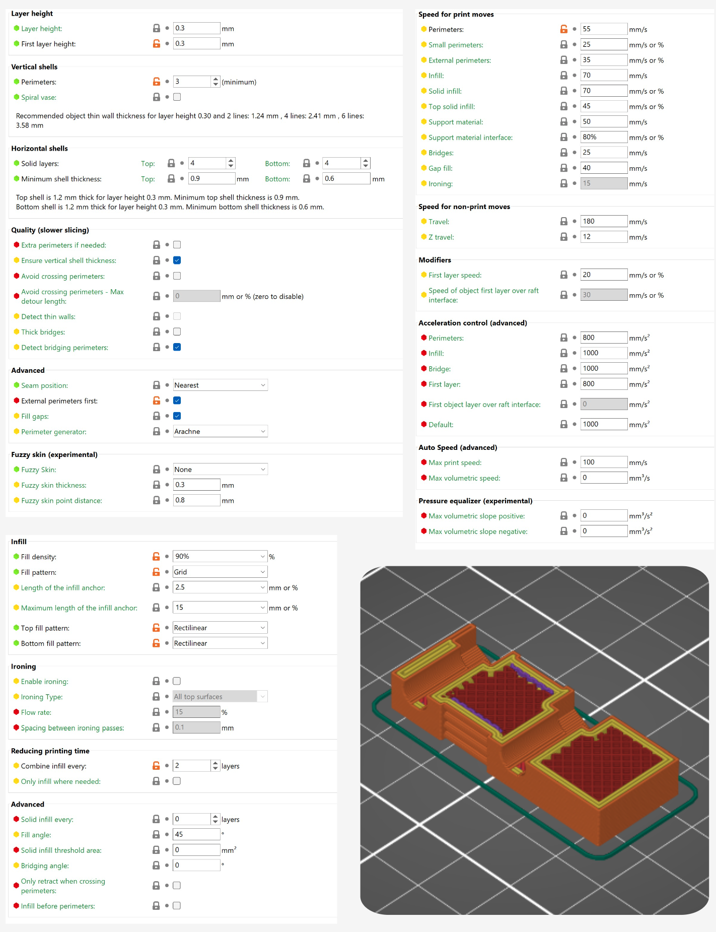
In the CAM tools for 3D Printing (known as slicers) users import 3D objects and set parameters to tune the process. Some parameters are geometric: layer height, track widths, external perimeter counts, and infill pattern and density. Other parameters set the machine’s speed (how fast the nozzle moves in cartesian space, also called translational rates) for different features: outside perimeters, interior perimeters, infill, etc. They select temperatures: for the nozzle, for the print bed, and (sometimes) for the print chamber. Finally, they adjust cooling parameters: slicers maintain a minimum layer time with the goal that when the next layer is printed, the previously deposited material is solidifying; this is important to avoid print slumping. All told, there are about one hundred parameters to tune in a slicer. Many of them need to be tuned for each new material, and more need to be tune when we change i.e. the nozzle diameter. Historically, tuning these parameters was a major barrier to the adoption of 3D Printing, but the community has over the years heuristically developed excellent presets for most commonly available materials and printers.
However, we need a new preset any time we change either the machine, the nozzle, or the material. It is becoming common also to develop a series of presets for each combination: one for “speed,” one for “quality,” and one for “strength”. This leads to a combinatorial explosion where the space of effective presets we would want explodes.
For example with a small set of only four machines, five materials, four nozzles, and three (speed, quality or strength) options we quickly arrive at 240 individual presets to develop. The world of FFF is in practice even broader than this: we have perhaps four machine companies at the top tier, nine ubiquitous materials (and versions of each with i.e. glass- or carbon-fiber fills), an ever-expanding frontier of new nozzle and hotend designs, and that speed / quality / strength tradeoff is in reality a continuous space of trade-offs. The preset solution limits adoption of each of these new innovations, leading users to stick with “tried and true” solutions even when superior options exist.
| Parameter | Typical Values | Units / Type | Physical Relation |
|---|---|---|---|
| Layer Height | \(0.1 - 0.4\) | \(mm\) | Geometry, Flow |
| Vertical Shells | \(2 - 6\) | count | Geometry |
| Horizontal Shells | \(3 - 6\) | count | Geometry |
| Infill | \(10 - 100\) | \(\%\) | Geometry |
| Infill Pattern | i.e ‘grid’, ‘gyroid’ | selection | Geometry |
| Shell Pattern | i.e. ‘rectilinear’ | selection | Geometry |
| Support Material | yes / no | selection | Geometry |
| Support Material Type | i.e. ‘grid’, ‘organic’ | selection | Geometry |
| Extrusion Widthsa | — | — | — |
| Default | \(d_{nozzle} \cdot 1.25\) | \(mm\) | Geometry, Flow |
| First Layers | \(d_{nozzle} \cdot 1.25\) | \(mm\) | Geometry, Flow |
| Perimeters | \(d_{nozzle} \cdot 1.25\) | \(mm\) | Geometry, Flow |
| External Perimeters | \(d_{nozzle} \cdot 1.15\) | \(mm\) | Geometry, Flow |
| Infill | \(d_{nozzle} \cdot 1.1\) | \(mm\) | Geometry, Flow |
| Solid Infill | \(d_{nozzle} \cdot 1.0\) | \(mm\) | Geometry, Flow |
| Top Solid Infill | \(d_{nozzle} \cdot 0.9\) | \(mm\) | Geometry, Flow |
| Support Material | \(d_{nozzle} \cdot 0.8\) | \(mm\) | Geometry, Flow |
| Speeds | — | — | — |
| Perimeters | \(25 - 250\) | \(mm/s\) | Motion, Flow |
| Small Perimeters | \(20 - 150\) | \(mm/s\) | Motion, Flow |
| External Perimeters | \(20 - 200\) | \(mm/s\) | Motion, Flow |
| Infill | \(50 - 350\) | \(mm/s\) | Motion, Flow |
| Solid Infill | \(20 - 250\) | \(mm/s\) | Motion, Flow |
| Gap Fill | \(20 - 100\) | \(mm/s\) | Motion, Flow |
| Bridges | \(10 - 50\) | \(mm/s\) | Motion, Flow |
| Support Material | \(10 - 100\) | \(mm/s\) | Motion, Flow |
| Support Interface | \(5 - 50\) | \(mm/s\) | Motion, Flow |
| First Layer | \(25 - 50\) (or as %) | \(mm/s\) | Motion, Flow |
| Travel | \(50 - 500\) | \(mm/s\) | Motion |
| Z-Travel | \(10 - 50\) | \(mm/s\) | Motion |
| Accelerations | — | — | — |
| Perimeters | \(1500 - 5000\) | \(mm^2/s\) | Motion, Flow |
| External Perimeters | \(1000 - 3000\) | \(mm^2/s\) | Motion, Flow |
| Infill | \(2000 - 10000\) | \(mm^2/s\) | Motion, Flow |
| Bridges | \(500 - 2000\) | \(mm^2/s\) | Motion, Flow |
| First Layer | \(100 - 1000\) | \(mm^2/s\) | Motion, Flow |
| Travel | \(2000 - 10000\) | \(mm^2/s\) | Motion |
| Travel (short) | \(100 - 1000\) | \(mm^2/s\) | Motion |
| Temperatures | — | — | — |
| Nozzle Temperature | \(160 - 300\) | \(^\circ C\) | Flow |
| Bed Temperature | \(40 - 120\) | \(^\circ C\) | Bed Adhesion |
| Chamber Temperature | \(40 - 80\) | \(^\circ C\) | Part Warping |
| Cooling Settings | — | — | — |
| Fan Enable Layer Time | \(5 - 50\) | \(s\) | Part Cooling |
| Minimum Layer Time | \(8 - 20\) | \(s\) | Part Cooling |
| Filament Settings | — | — | — |
| Maximum Flowrate | \(10 - 50\) | \(mm^3/s\) | Motion, Flow |
| Extruder Settingsb | — | — | — |
| Retraction Length | \(0 - 5.0\) | \(mm\) | Motion, Flow |
| Retraction Speed | \(10 - 100\) | \(mm/s\) | Motion, Flow |
| Deretraction Extra Length | \(0 - 1.0\) | \(mm\) | Motion, Flow |
| Deretraction Speed | \(5 - 50\) | \(mm/s\) | Motion, Flow |
a I’ve included extrusion widths here as a function of nozzle diameter \((d_{noz})\) but they are often also calculated with respect to layer height; if we try to extrude i.e. a 0.2mm track width at a 0.4mm layer height, the track does not connect to the previous layer. These are not a commonly re-tuned value, as defaults are easy to arrive at using those known variables.
b Settings for retracts can be tuned in two places: connected to the machine (which may have an amount of baseline extrusion slack) and as an “override” in the filament related settings, for i.e. very flexible filaments that may require extra retraction.
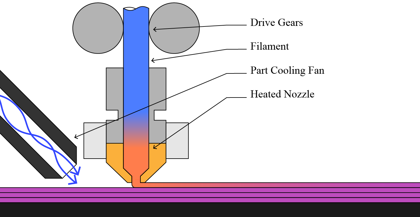
The values we set in slicers all relate explicitly to the machine instructions (how fast to travel, how thick to make the layer, etc). They relate implicitly to the physics of 3D printing, which has mostly to do with flow rates and temperature of the polymer melt (see Figure 6.2 below and Section 6.5 for a more complete description of FFF physics) (Mackay 2018). Table 6.1 (above) lists the most important slicer parameters, and how each relates to our control task. A subset are related to part geometry only, but most relate to at least two aspects: flow and geometry, flow and motion, etc.
For example if we double the layer height but retain the same speeds we double the flowrate of the polymer melt: this has huge ramifications for the physics of the process, but that is not reflected anywhere else in the parameter set. Manually changing print speeds to reflect the new layer height would mean updating nine other parameters (excluding those that can be set by a percentage). Nor are those parameters related to longer-term outcomes like the resulting thermal history of the print’s inter-layer joints, which are a main indicator of part strength (Coogan and Kazmer 2020). Inversely, if we increase the nozzle temperature we often unlock more flow rate, but there is no way to update print speeds as a function of temperature, or increase layer cooling time. Instead of having any knowledge of print physics built into the slicer, users need to intuit how these many parameters will relate to the machine’s operation.
6.3 The Proposed FFF Workflow
Conceptually, this workflow operates in two steps: machines make models, and we then combine those with heuristics to operate the machine. Below, Figure 6.3 shows this process in more detail.
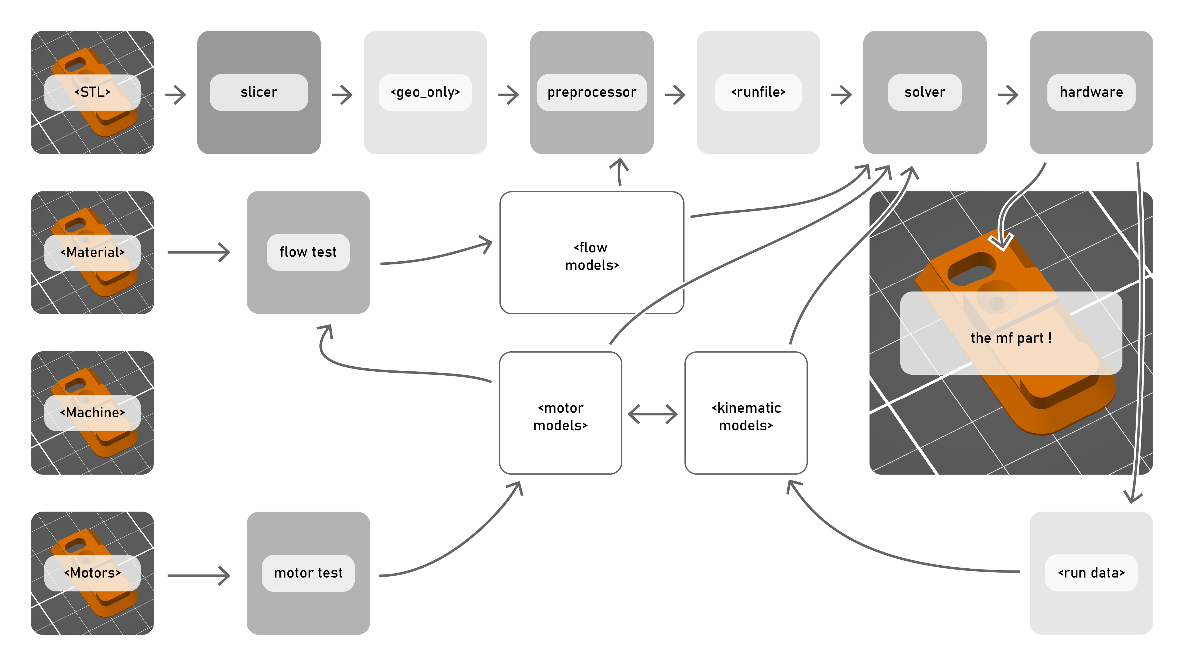
Rather than setting low-level parameters explicitly, this workflow uses models to pick those parameters. I do not take on the task of generating path geometry, instead focussing mostly on the parts of the problem that combine motion and flow optimizations, i.e. speed selections. While geometry and motion are of course coupled in reality, we can safely generate one part geometry and print it in multiple materials so long as we adjust our rates accordingly.
The workflow is similar to the state of the art, but with some key differences. It first requires that we generate some models: for flow, cooling, and for our machine. These steps are described in Section 6.5, Section 6.6 and Section 6.7. Then we follow this sequence:
- The desired part file is turned into a path file, where we can select layer height, infill densities and patterns, and shell thicknesses. This is a static path encoding that contains a series of path segments and widths, each segment of which is binned into one of five categories: infill, perimeter, small, outer, and travel moves.
- The preprocessor (Section 6.8) is configured with material flow and cooling models, as well as user heuristics for motion, flow and cooling, and some estimates (see Table 6.5). It selects an optimal nozzle temperature for the combination and generates a run file, which is an annotated version of the path file whose data are described in Table 6.3.
- The run file is passed to the solver, (Section 6.9) along with motor, motion, and flow models. The solver optimizes real-time control outputs to the machine to execute the job - maximizing speed while respecting constraints laid out in the models and in the run file. It is connected to the machine via OSAP (Chapter 2), Pipes (Section 3.2) and MAXL (Section 3.3).
- During the print, time series data are collected from the machine and it’s instruments and stored in a run data file. This data can be used to improve models, detect errors, or analyse machine performance.
| Preprocessor Input | Units | Typ. | Mediating Models | Destination |
|---|---|---|---|---|
| Cooling Estimates | — | — | — | — |
| Chamber Temp | \(^\circ C\) | \(30.0\) | Cooling | Preprocessor |
| Cooling Target \(\Delta T\) | \(^\circ C\) | \(-20.0\) | Cooling | Preprocessor |
| \(h_{air}\) est. | \(5.0\) | Cooling | Preprocessor | |
| \(\kappa_{fil}\) est. | \(0.1\) | Cooling | Preprocessor | |
| Straight Heuristics | — | — | — | — |
| First Layer Rate | \(mm/s\) | \(50.0\) | Both | |
| Minimum Flow | \(mm^3/s\) | \(15.0\) | Flow | Preprocessor |
| Pressure Scalars | — | — | — | — |
| Infill | \(0-1.0\) | \(0.75\) | Flow | Both |
| Perimeters | \(0-1.0\) | \(0.65\) | Flow | Both |
| Details | \(0-1.0\) | \(0.45\) | Flow | Both |
| Current Scalars | — | — | — | — |
| XYZ (fast) | \(0-1.0\) | \(0.20\) | Motion | Solver |
| XYZ (fine) | \(0-1.0\) | \(0.25\) | Motion | Solver |
| E (fast) | \(0-1.0\) | \(0.75\) | Motion, Flow | Solver |
| E (fine) | \(0-1.0\) | \(0.60\) | Motion, Flow | Solver |
| Current Slew Rate Scalars | — | — | — | — |
| XYZ (fast) | \(0-1.0\) | \(0.125\) | Motion | Solver |
| XYZ (fine) | \(0-1.0\) | \(0.110\) | Motion | Solver |
| E (fast) | \(0-1.0\) | \(0.50\) | Motion, Flow | Solver |
| E (fine) | \(0-1.0\) | \(0.50\) | Motion, Flow | Solver |
| Extruder Heuristics | — | — | — | — |
| Pressure Offset | \(N\) | \(15.0\) | Solver | |
| Reset Balance | ratio | \(0.80\) | Solver | |
| E Rate Limit | \(mm^3/s\) | \(75.0\) | Solver | |
| E Acceleration Limit | \(mm^3/s^2\) | \(40000.0\) | Solver |
| Run File Content | Units | Notes |
|---|---|---|
| Per-Segment Variables | — | |
| Max Overall Rate | \(mm/s\) | Enforced for part cooling and flow heuristics. |
| Max XYZ Current Deployment | \(0-1.0\) | |
| Max E Current Deployment | \(0-1.0\) | |
| Max XYZ Current Slew Rate | \(0-1.0\) | |
| Max E Current Slew Rate | \(0-1.0\) | |
| Fixed Variables | ||
| Nozzle Temperature Setpoint | \(^\circ C\) | |
| Retract Target Pressure | \(N\) | |
| Retract Reset Assymmetry | \(0.0-1.0\) |
At first glance it might look like we replaced one set of parameters (Table 6.1) with another (Table 6.5), but in our workflow the heuristics are mediated by models: flowrates are set by targetting an allowable pressure that is scaled by the flow model, and motion (speed and acceleration together) is scaled via the motion model, by specifying how much current the machine should be allowed to deploy for different parts of the path. Whereas the state of the art workflow requires us to re-tune parameters for any change to the machine, material, or nozzle, here we can instead modify the underlaying models and cast the same set of heuristics through them: the preprocessor and solver work together to adjust real-time control outputs accordingly.
6.4 Hardware
In order to develop and deploy this new workflow, we are going to need some hardware. In this section I will explain the two machines I developed for this chapter: the first was my development mule, the second is a minimally modified off-the-shelf machine.
6.4.1 The RheoPrinter
The RheoPrinter is a custom built machine for the purposes of this project. The hardware is representative of most commercially available FFF 3D Printers, except for the addition of instruments in the hotend, as detailed in the figure above.
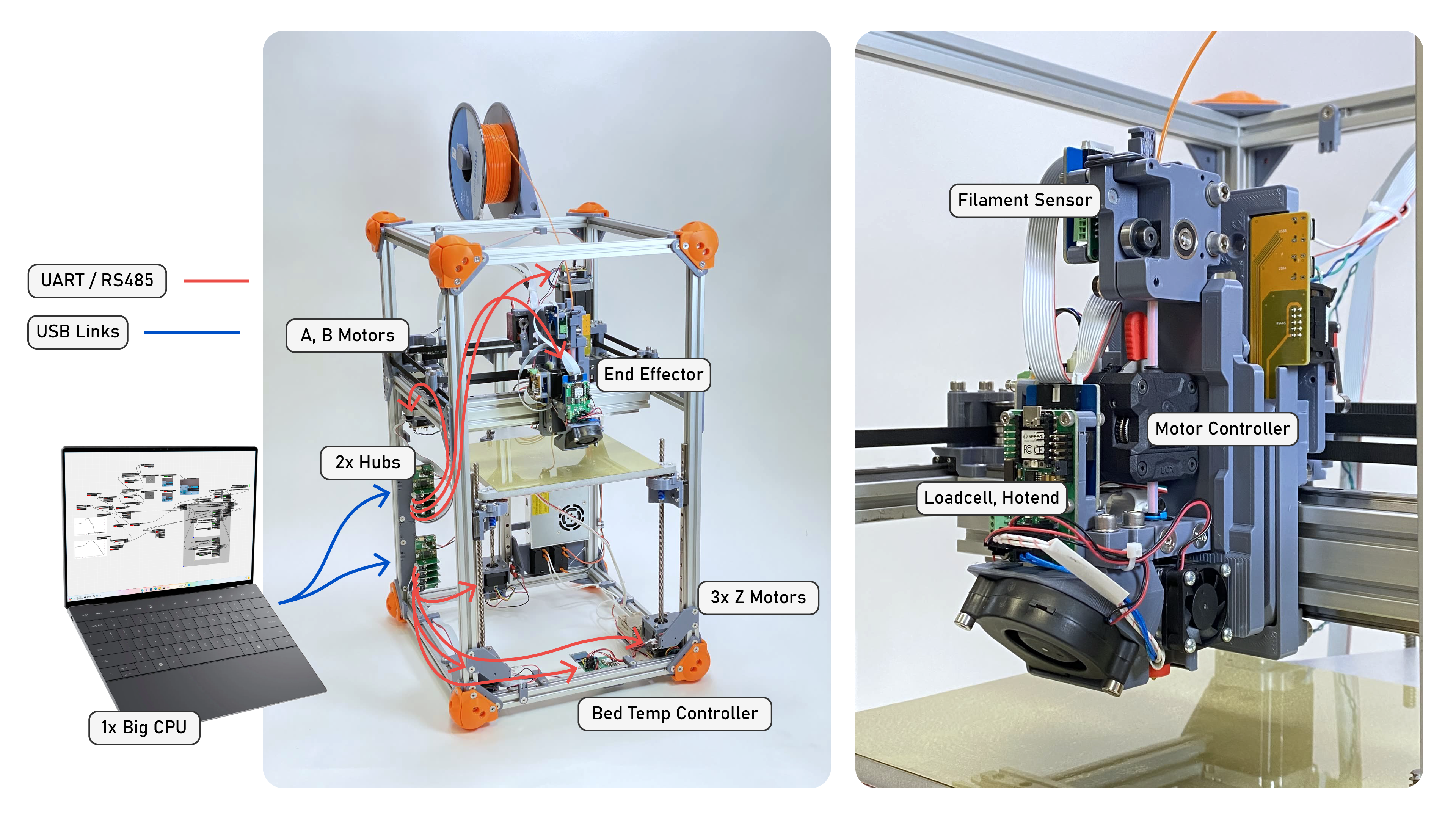
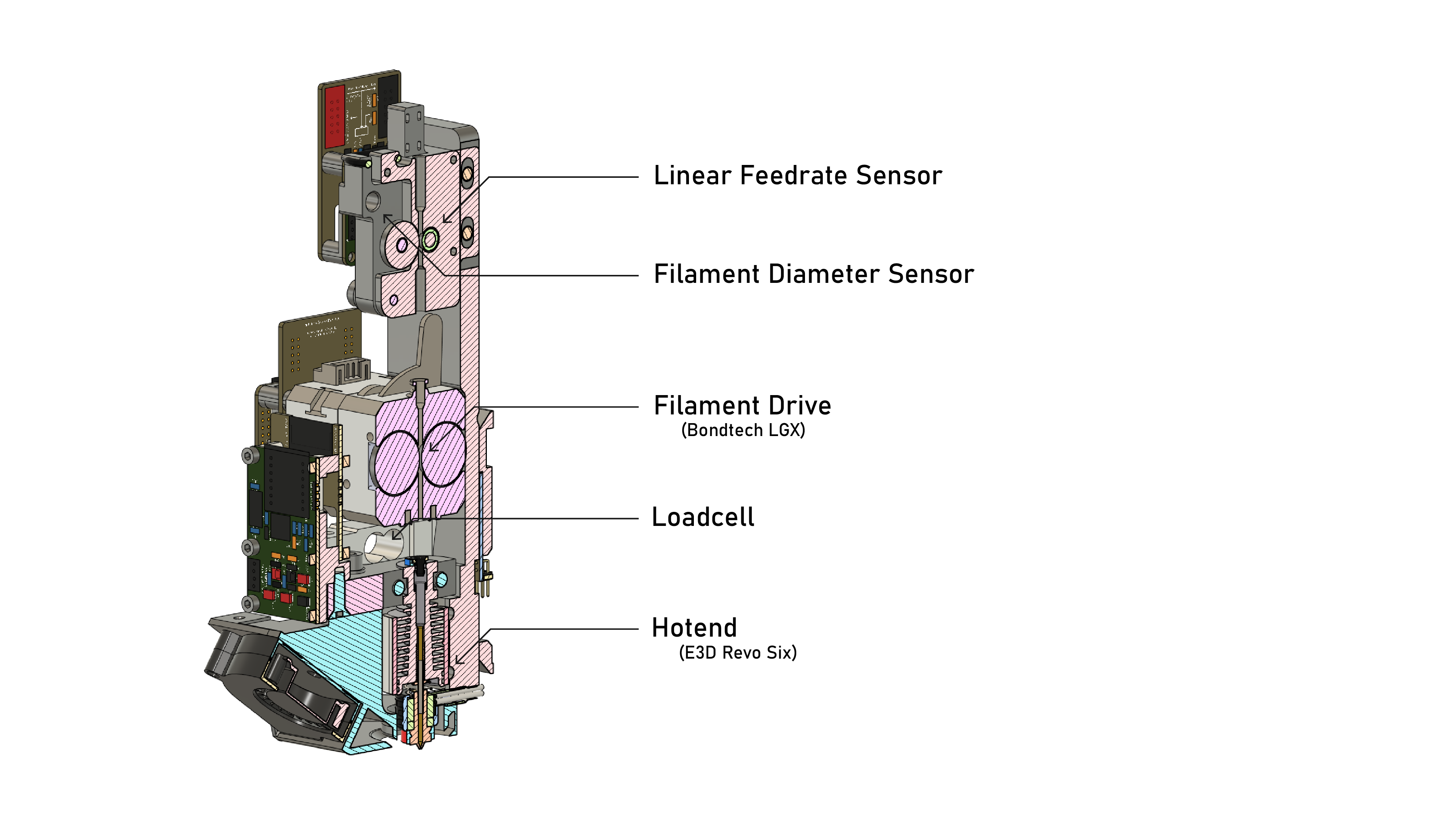
I originally included a Linear Feedrate Sensor on the machine to detect changes to filament width and slip between the extruder drive gears and filament. Use of this instrument is not outlined in this thesis; it became mostly redundant once the extruder motor models were sufficiently well developed.
6.4.2 The FrankenPrusa
While the hardware on the RheoPrinter has a similar mechanical architecture to state of the art printers, the particular implementation is of course different than any off-the-shelf printers available. Motors are larger with more rotor inertia, axes are heavier, and of course the friction values are different. It also uses an extruder and hotend combination that (while commercially available) is not implemented in any particular off-the-shelf machine.
In the evaluation of this printing workflow we are interested in comparing just this control system with the state of the art. To do this without having to dissect which differences arise from actual hardware limits, I retrofit a Prusa Core One (“Prusa Core One” 2024) with my own control boards (Chapter 4).
This involved fitting motor and kinematic models of the printer using the workflow I described in Section 5.3.1 and Section 5.3.2, and then fitting flow models using techniques described in this section. The lynch-pin for me here is that the Prusa print head (dubbed the Nextruder (“Prusa Nextruder” 2024)) implements a loadcell into its design - primarily used by them for bed leveling - this is not available on all SOTA printers, but it is the most important flow modeling tool in our kit.
Besides the loadcell, I also added a microbolometer to the Prusa, since time series thermal data is invaluable in print analysis (but not required for the work described here). All other sensing is done either with thermistors or with motor controller current measurements. For more detail on the retrofit process itself, see Chapter 4.
Using this hardware, our comparisons bear more weight as we know that the ground truth physical constraints in our system are identical to those used by Prusa. It also gives us a set of print parameters to compare against, as they do an excellent job of shipping expertly tuned slicer parameter sets for their hardware.
6.5 Models for FFF Flow
This section starts with a brief explanation of polymer melt flow physics (below) and covers relevant background on the topic (Section 6.5.2). I then develop a series of models and model fitting routines. This includes steady state models in Section 6.5.3 and isothermal / dynamic models in Section 6.5.4. In practice flow is neither steady-state or isothermal, and so I develop a strategy to interpolate between these two models in Section 6.5.5.
This is an important set of methods in our work; models must have enough fidelity to capture the important physics, should also be simple enough to fit easily on the available data and to run near real-time in the machine’s motion controller. Models are evaluated in Section 6.10.1 by reporting model errors for real world prints (comparing the solver’s pressure predictions to measured nozzle pressures), and in more detail in Section 6.10.2.
6.5.1 FFF Flow Physics Overview
To my immeasurable dissappointment, polymer extrusion is a deviously confounding system to model. See Figure 6.2 (and caption) for an overview of the system. In total, probably one or two years’ worth of work in this thesis was done only on this topic: trying to understand it intuitively, and then trying to build fitting routines and mathematic models of that understanding that would suitably fit to data, and which are robust and simple enough to use as control components.
In building predictive flow models, we are trying to understand what flowrate will emerge from the tip of the nozzle at any given time (I will use \(Q_{out}\) for this value, in \(mm^3/s\)), at any given nozzle temperature and pressure. The value depends on a handful of inputs, which I enumerate below.
- The polymer has a viscosity that is dependent on it’s temperature and shear rate (i.e. nozzle pressure) - polymers actually become less viscous when they are under pressure (this is called shear thinning).
- The filament between the extruder’s drive gears and the nozzle is compressible, and so we must build pressure before extrusion begins and measure the stiffness of the material (that stiffness also changes with temperature).
- The extruder motor has its own dynamics that must be coupled into the flow system.
- The thermal history of the filament in the melt zone needs be considered: filament takes time to come up to the nozzle’s temperature and at high extrusion speeds the melt flow does not reach this temperature before it is extruded, leading to colder flows where we need more pressures to achieve the same flowrate.
6.5.2 Other Research on FFF Flow Modelling
Luckily there is a lot of interest in FFF printing in the literature, and so the applied physics are quite thoroughly understood (Turner, Strong, and Gold 2014) (Mackay 2018).
Of particular relevance to this work is a line of research begun by TJ Coogan and David Kazmer, who developed an instrumented extruder similar to ours in (Coogan and Kazmer 2019). Filippos Tourlomousis takes credit for bringing this idea to the CBA and implementing the first version of the hardware, and I extend a design pattern developed by an FFF youtuber to implement the filament sensor (Sanladerer 2021) (adding a feedrate encoder, and calibrating width measurements). Kazmer continues work to characterize the dynamic behaviour of filament during extrusion in (Kazmer et al. 2021), which helped me to develop the dynamics model I use in the current iteration of the FFF flow model. These works were also fundamental to my work in (Read et al. 2024) (see Figure 6.9), where we combined online model-building with parameter selection in a reduced space to print with unkown materials.
A selection of the literature disccusses performance limits to FFF printing, notably (Go et al. 2017) discusses absolute limits to print speeds based on nozzle thermodynamics and (Mackay et al. 2017) models flowrates through a hotend as a function of nozzle temperature. The focus of the work in this thesis is not necessarily to push those limits, but to develop controllers that more routinely run at or near those limits (pushing performance of existing systems).
Another selection studies the relationship between slicer settings and print performance (strength, precision) (Afonso et al. 2021) (Deshwal, Kumar, and Chhabra 2020) (Qattawi et al. 2017) (Luzanin et al. 2019) (Ferretti et al. 2021), but these studies all operate in an outer loop around the state of the art workflow - i.e. they optimize slicer parameters, whereas (as I discussed in Section 6.2) these are a somewhat lossy abstraction over the as processed parameters (due to firmwares’ speed scaling).
Researchers are also interested in modelling inter-layer weld strength (Coogan and Kazmer 2020) (Davis et al. 2017), which is a function of the weld’s thermal history (more time above the plastic’s glass transition temperature equates to more diffusion of polymer chains across the weld), and the inter-layer pressure exerted by the pressure during extrusion. It should be possible using the framework developed in this thesis to describe those physics as an optimization target, for example adding to the solver’s cost function a reward for maximizing weld temperature - but doing so would probably involve much more complex simulation of the print as a whole, whereas my approach only considers shorter time spans.
Despite all of this research, there is limited literature that combines rheological modeling with online controllers and motion systems - except for (Wu 2024). They make significant progress in adapting online control to optimize extrusion during machine operation, using flow models fit from line-laser scans in conjunction with servo control of the extruder motor in a hybrid system, eliminating many extrusion defects like under- or over-extrusion. To compare with work in this thesis, our approach combines similar models for extrusion with more advanced models of machine motion and kinematics, which should yield overall improvements to print speed - taking the machine system as a whole, whereas their work focuses mainly on the optimization of extruder commands. Ours also integrates the additional loadcell and filament sensors, which allows us to bootstrap models on previously unseen filaments.
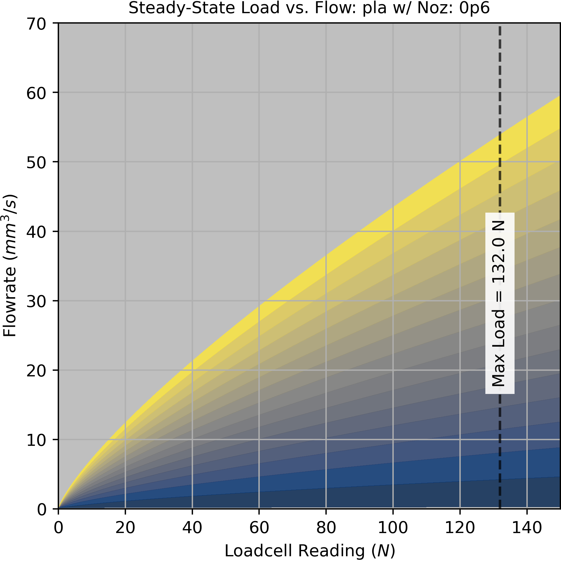
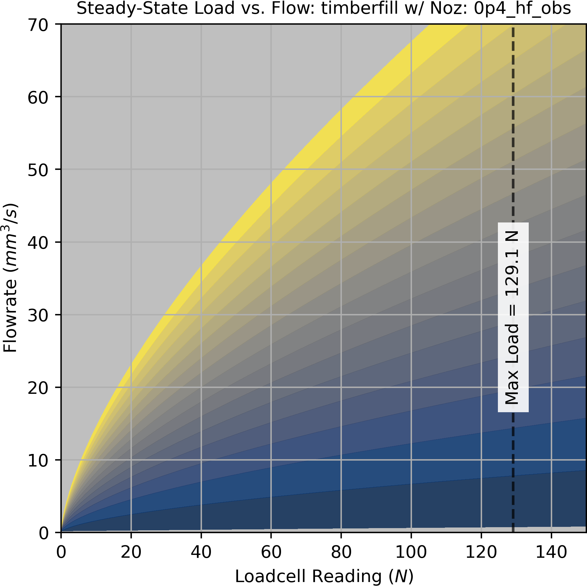
6.5.3 Steady-State Flow
Given that we start with little or no information about our system (besides the motor model), our first modelling challenge is to find the maximum flowrate that can be achieved at any given temperature. This will set an initial boundary for operation within which our tests for dynamic models can be performed without fear that we will operate the machine in a failure mode; we want our tests to be non-destructive, so that we can proceed without having to manually reload or reset filament, etc.
I developed a simple open loop test for this that is quick, repeatable, and provides us with enough information to determine a few key parameters: (1) a linear fit for maximum flowrate across temperatures, which includes (at the zero crossing) what I call the “zero flow temperature” which is the coldest point at which we can expect any flow to be possible, and (2) a nonlinear fit that gives us the expected nozzle pressure at any steady state flowrate and nozzle temperature. The data from this test is also used (3) to estimate the filament’s volumetric heat capacity, which can be used in conjunction with simple cooling models to generate minimum layer times (more on those later).
1. Heat the nozzle to its maximum temperature.
2. Set the extruder's velocity controller setpoint to our test rate.
3. Turn the nozzle heater off.
4. While the velocity controller's error is below some threshold:
  - Collect time series data for:
    - Loadcell Force
    - Extruder Motion States
    - Nozzle Temperature
    - IR Frames
5. Restart the test at the next flowrate.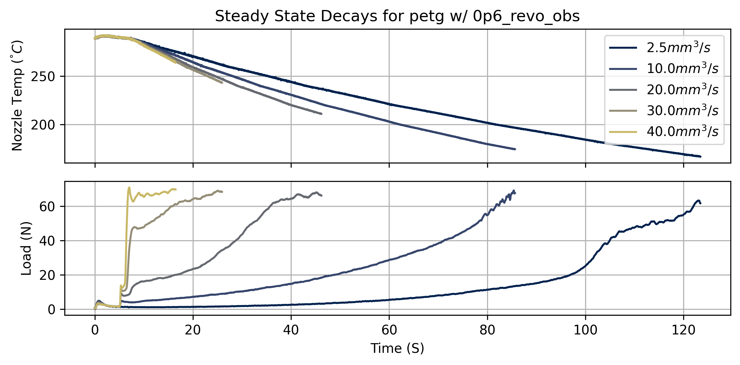
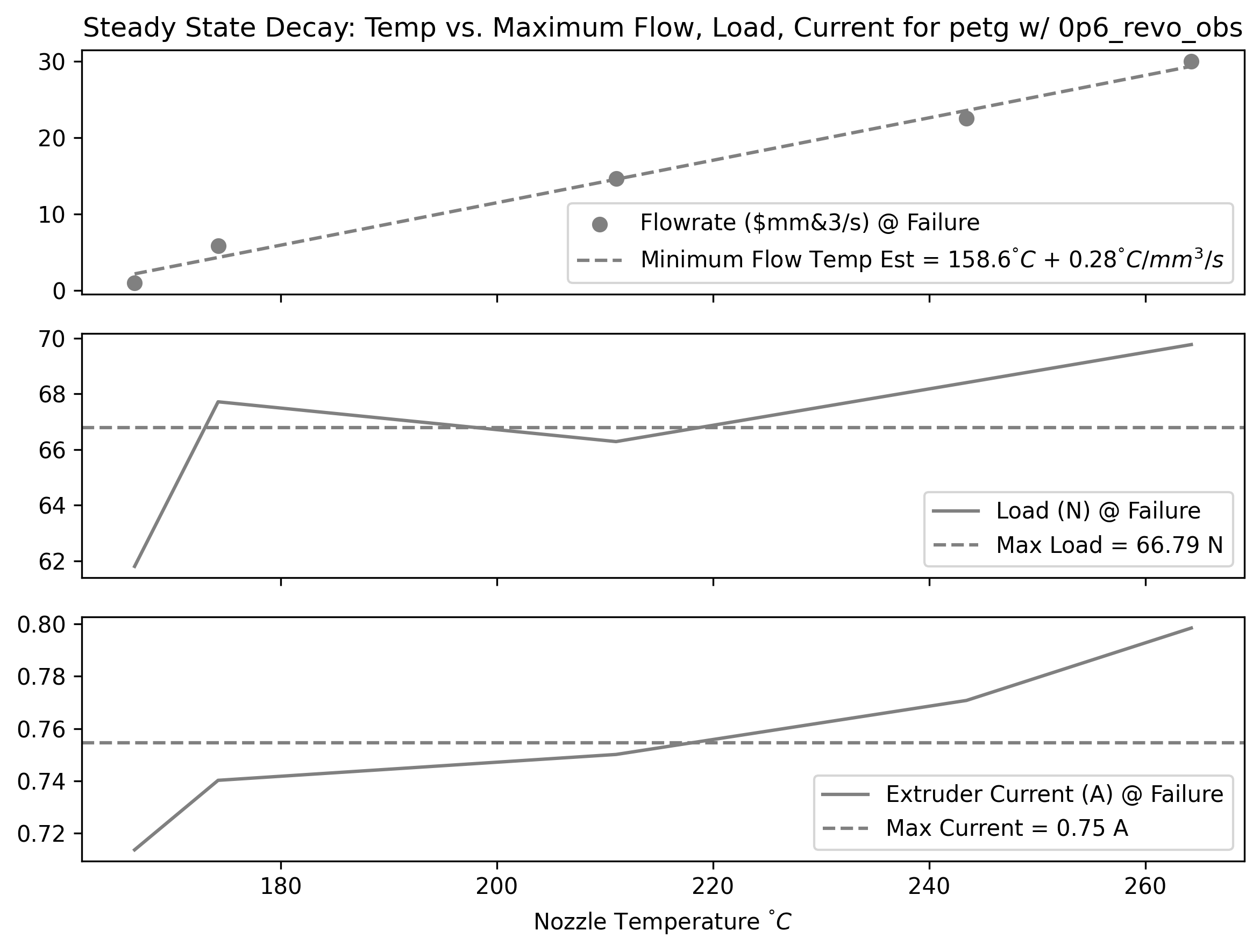
By measuring the temperature, loadcell, and motor current readings at the failure points for each test, we can extract simple estimates for the system’s maximum pressure and current across temperatures.
We can also fit a linear model for the minimum flow temperature across flowrates. The zero crossing of this linear fit is an estimate of the nozzle temperature where we might expect any flow to be possible; I call this the zero flow temp, or \(T_{min}\) - which we will use to normalize temperature ranges in some of the next steps’ fits.
In steadystate, our system is basically limited by the force we can exert on the filament, i.e. the pressure we can generate in the nozzle. In order to pick an operating region, we want to understand the relationship between nozzle temperature, pressure, and the resulting flowrate. So, some function:
\[ Q_{ss} = f_{ss}(F, T) \tag{6.1}\]
- \(Q_{ss}\) is steady-state flowrate (\(mm^3/s\))
- \(F\) is the loadcell reading (N)
- It is important to note that this is a pressure analog, not a direct pressure measurement. Reducing this measurement to a real nozzle pressure is presumably simple, but internal nozzle geometries vary by manufacturer, and an exact pressure measurement is not useful for our purposes of finding machine operating points (although it would be valuable if we wanted to deduce real viscosity measurements from our system).
- \(T\) is the nozzle setpoint temperature (\(^\circ C\))
- Recall that this is not exactly related to the melt flow temperature, which may be substantially colder than the nozzle (especially at large flowrates, where the material does not dwell in the nozzle for long).
At a single temperature, Equation 6.2 does well to model the relationship.
\[ Q_{ss} = f(F) = (F \cdot k_{ss,lin}) ^ {k_{ss,pow}} \tag{6.2}\]
To broadcast that across temperatures, we can fit additional parameters that vary across a normalized temperature band which. When these models are fit, we also fit \(T_{min}\)
\[ \begin{aligned} T_{norm} &= \frac{T - T_{min}}{T_{max} - T_{min}} \\ k_{ss,lin} &= T_{norm} \cdot a + b \\ k_{ss,pow} &= T_{norm} \cdot c + d \\ \end{aligned} \tag{6.3}\]
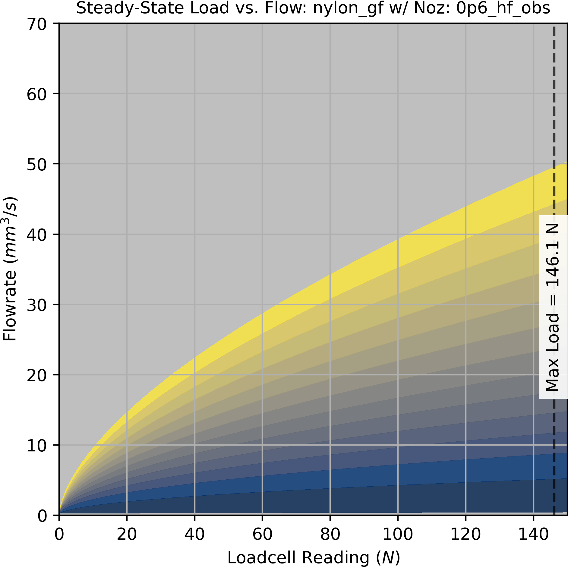
Using these together, we have our complete \(Q_{ss} = f_{ss}(F, T)\) to model steady-state flow for a given temperature and pressure.
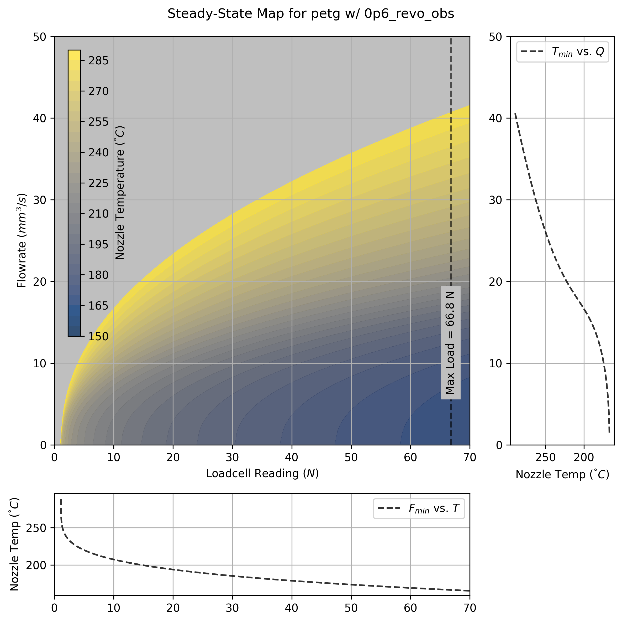
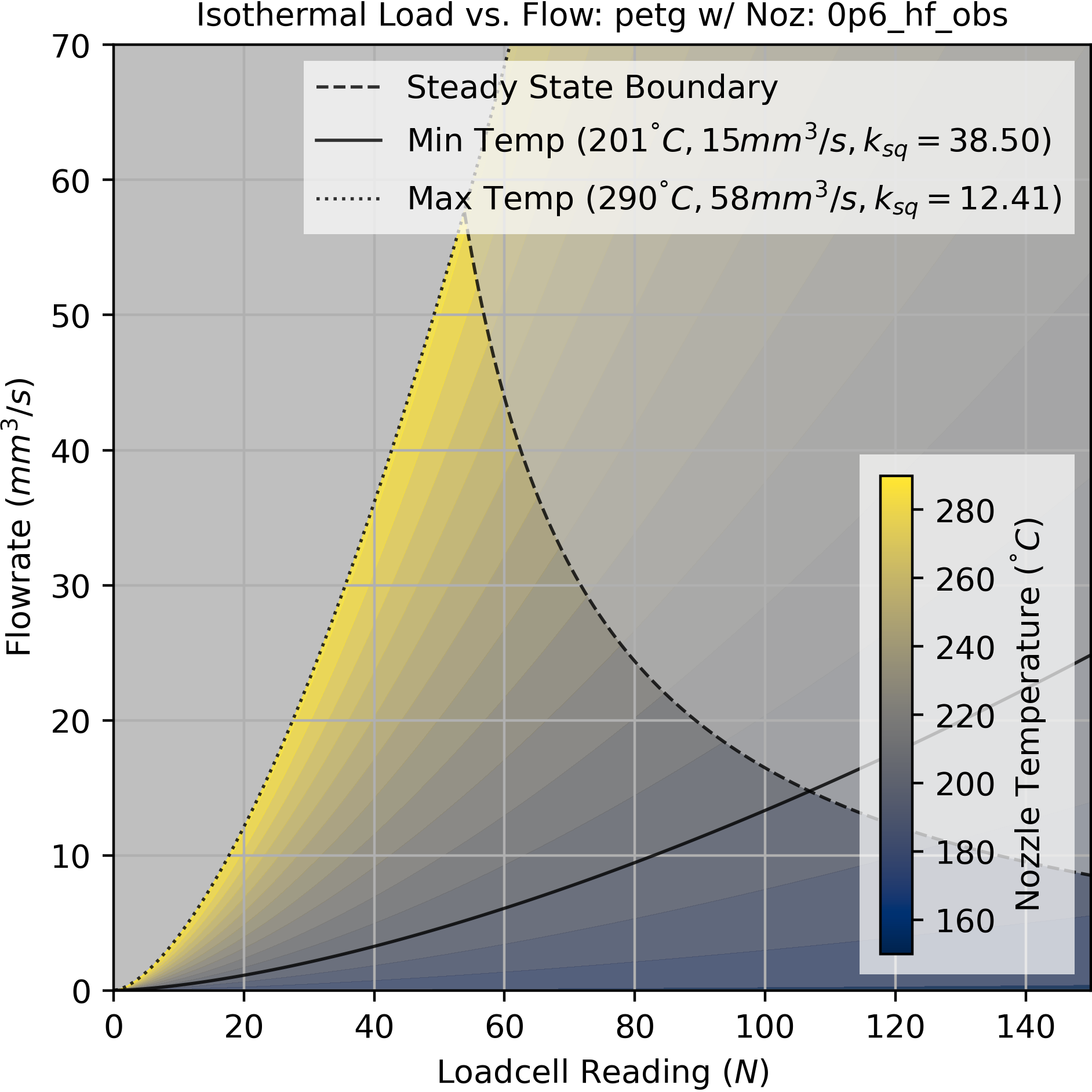
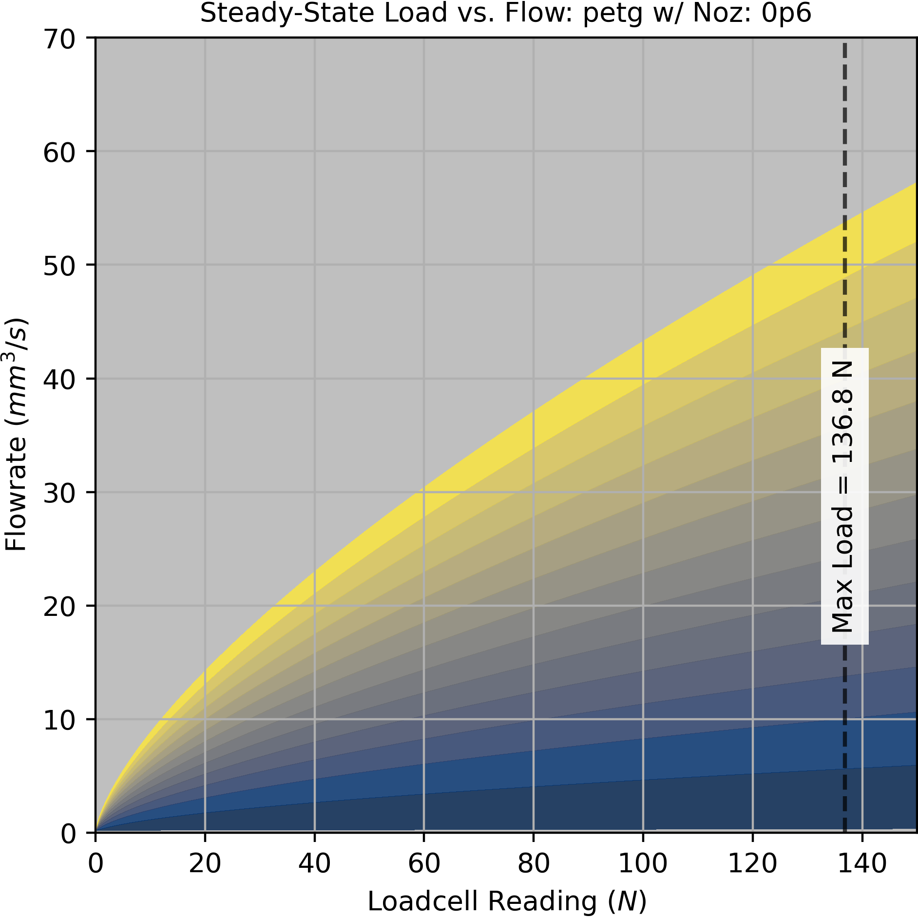
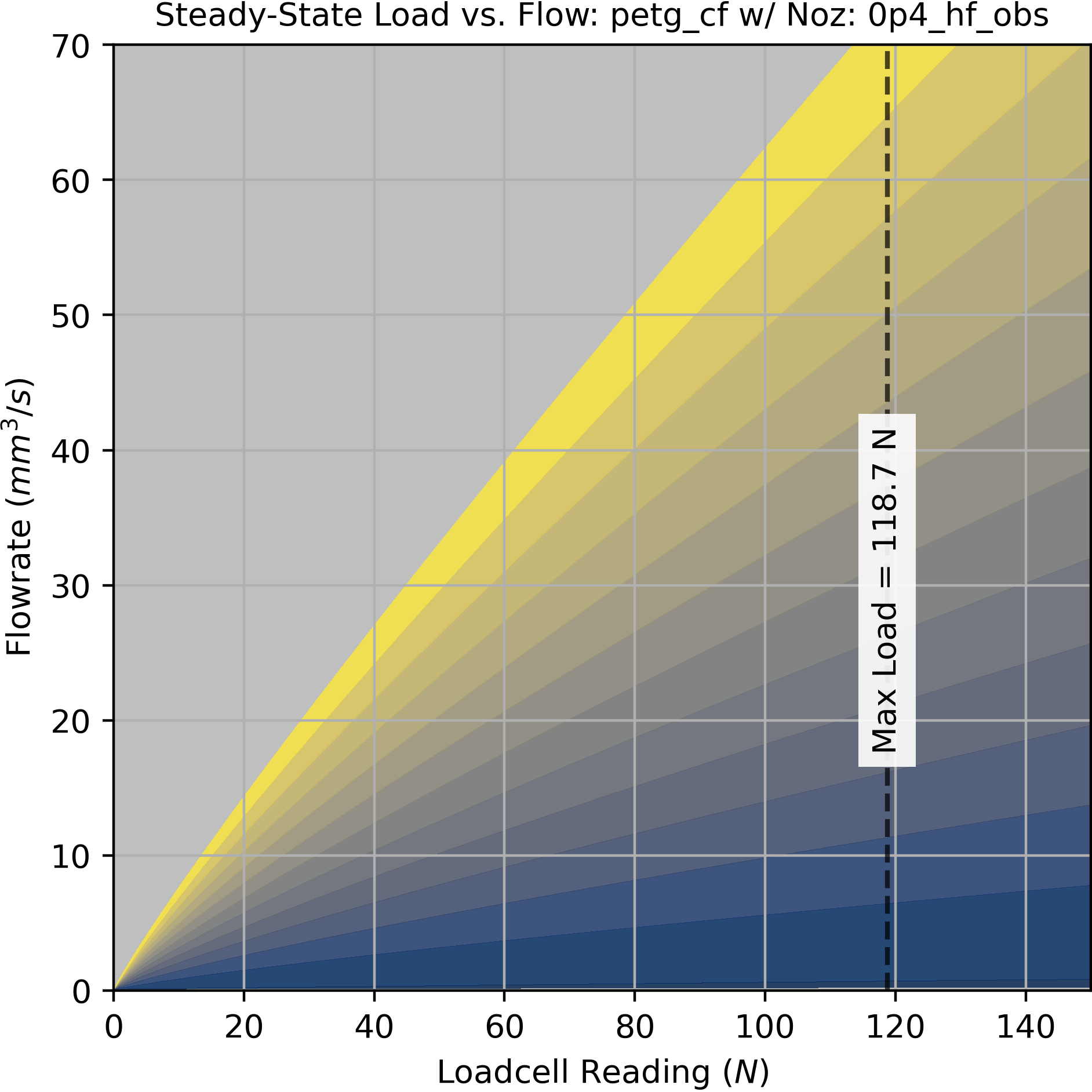
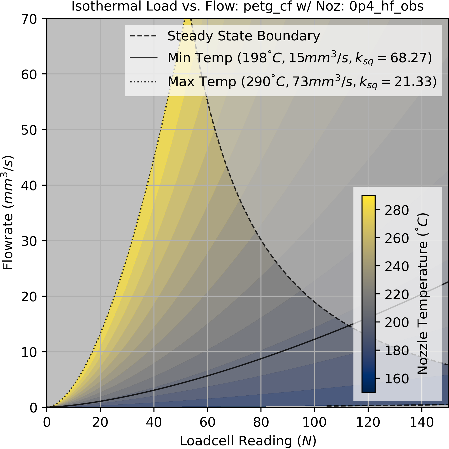
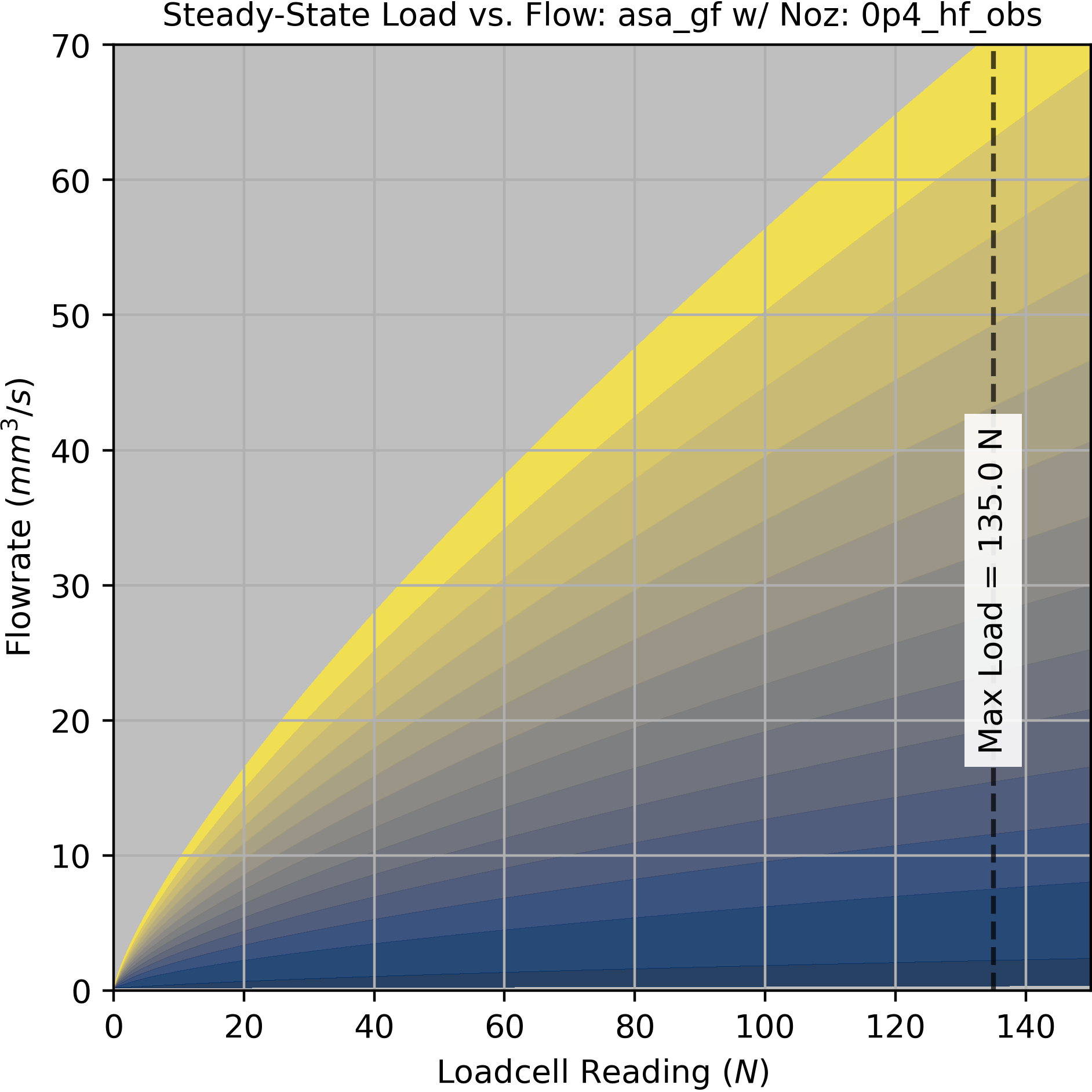
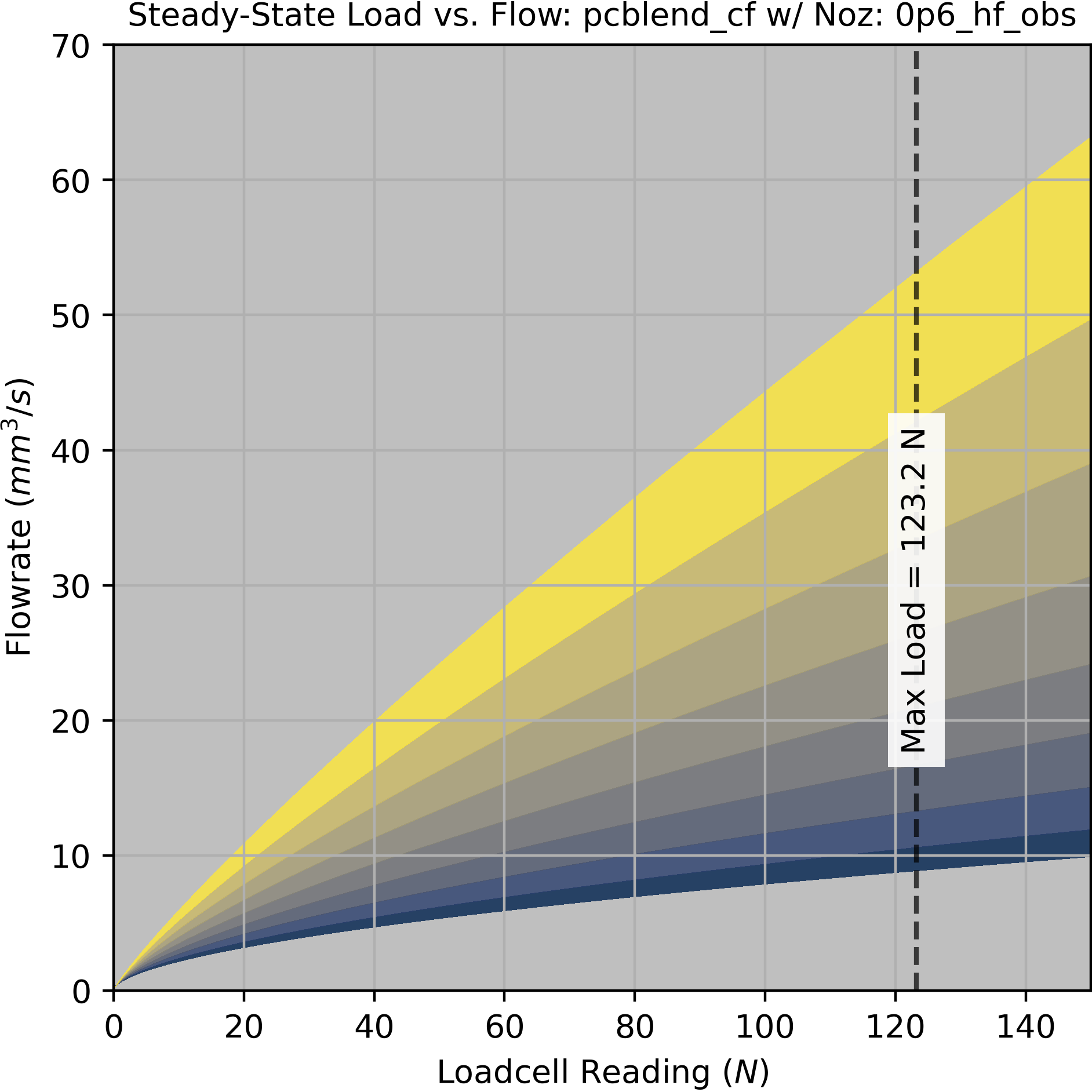
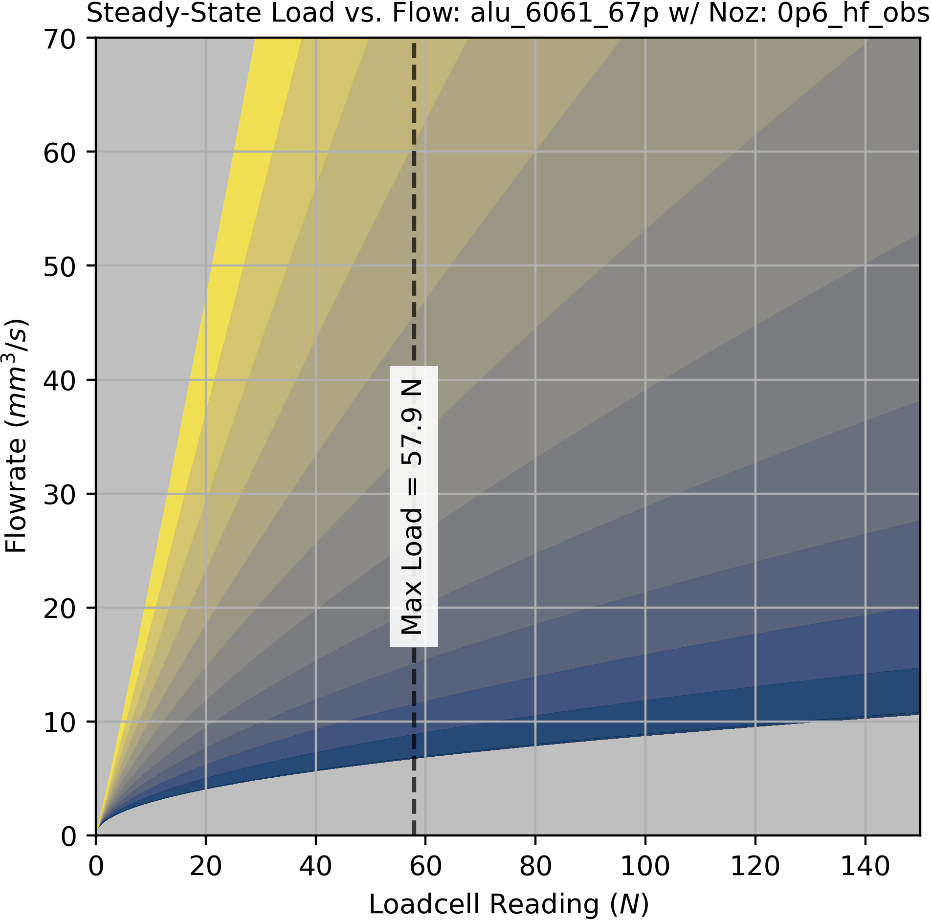
The map is not exactly a physical model, but we can extract some useful information from it. A slice through the maximum extruder load value sets a boundary for our dynamic operation, i.e. a maximum flowrate across a range of temperatures. We use this slice to set a boundary on our dynamic map in the next subsection (see Fig. Figure 6.10). A slice through zero flowrate shows us the deadband pressure across temperatures.
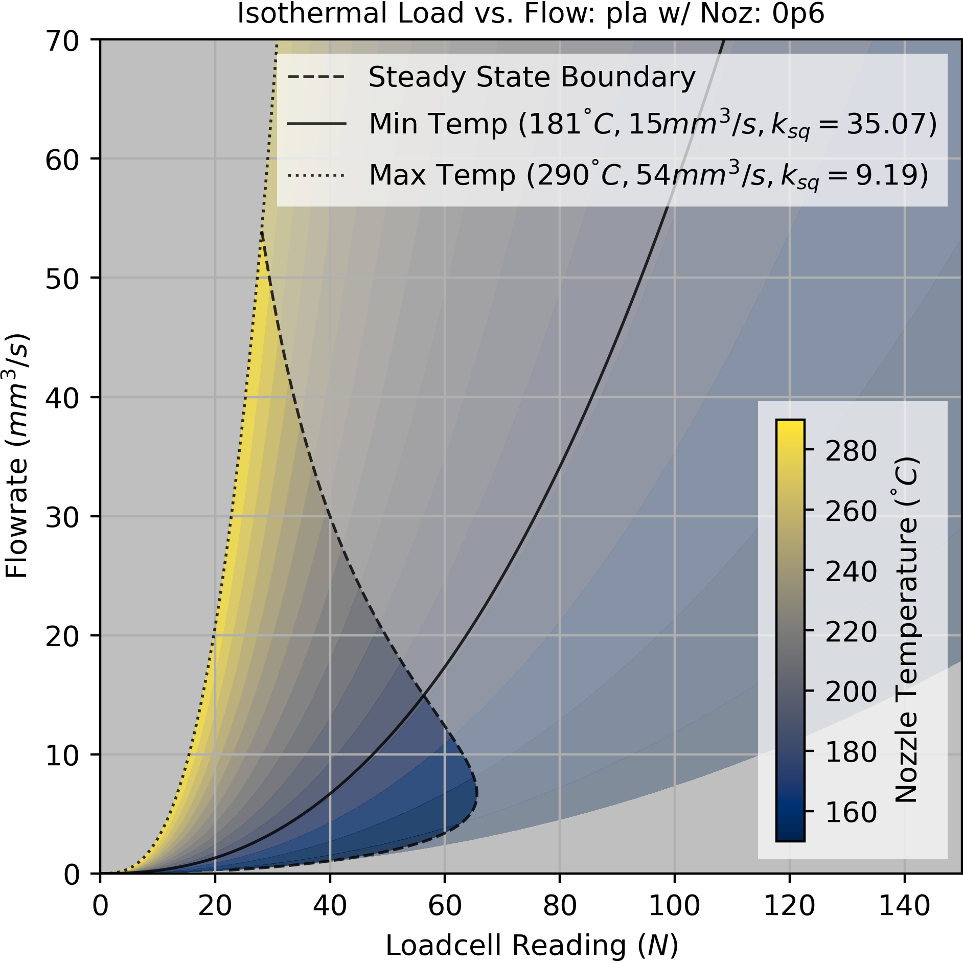
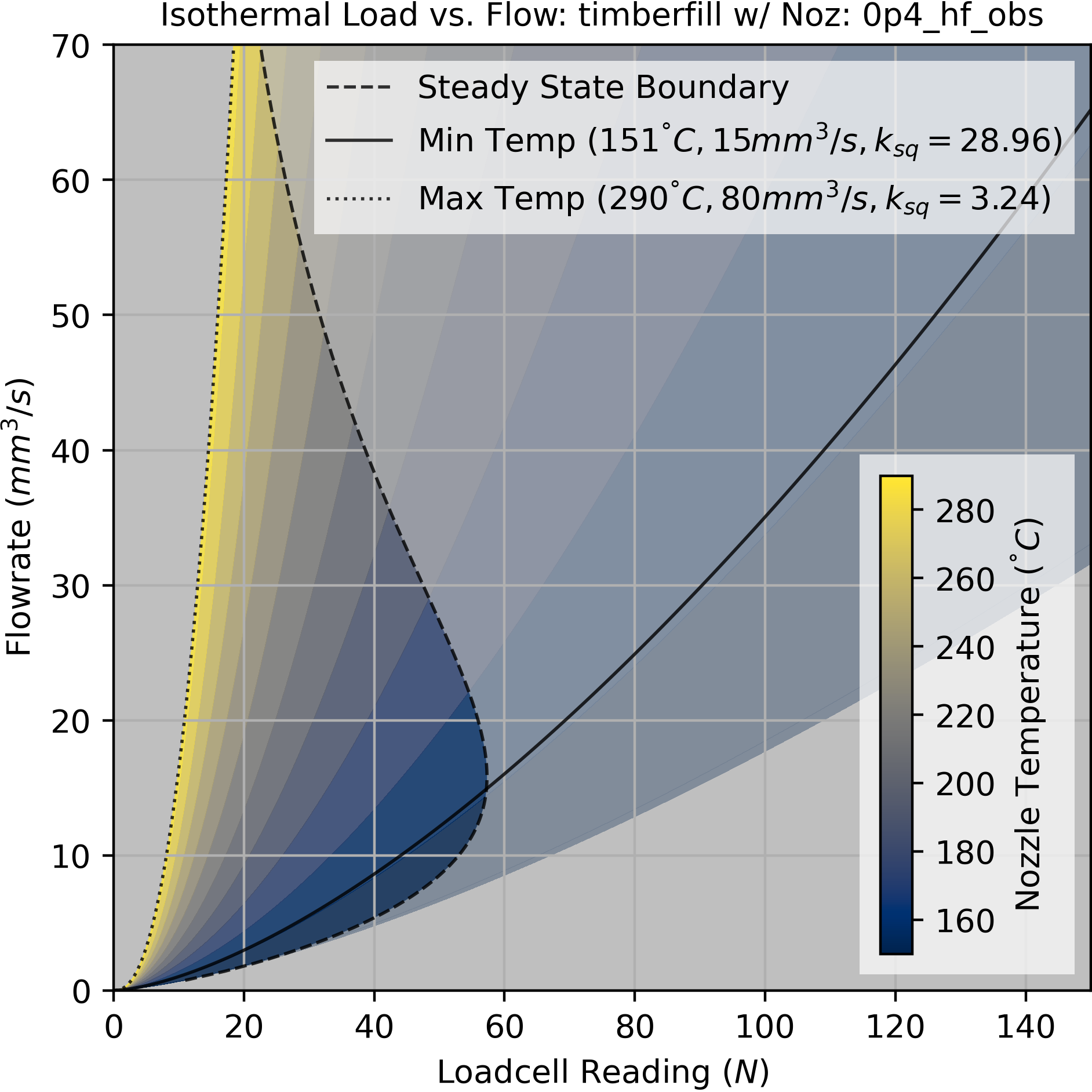
6.5.4 Isothermal Flow and Compression
The steadystate model helps us to set operating boundaries for our machine, but it does not properly model operation of the system during short time intervals. In practice, most FFF printing is dynamic: machines are constantly accelerating and deccelerating and flow targets are correspondingly increasing and decreasing such that track widths remain consistent.
Recall in Fig. Figure 6.2 that the filament between the drive gears and nozzle tip acts as a spring: this means that we need to anticipate increases to extrusion rate by preloading this spring, and anticipate reductions to extrusion rate by unloading the spring. This is handled approximately in state of the art printer firmwares approach called linear advance (Research, n.d.). However - this is a firmware setting. Not all controllers allow this to be modified without re-compiling a firmware, and those that do allow this need the slicer to tell them where to set it. Filament compressibility is not just dependent on the filament (whose stiffnesses vary wildly), but on the printer design (some have better extruder designs than others) and the flow temperature (warmer melts are squishier).
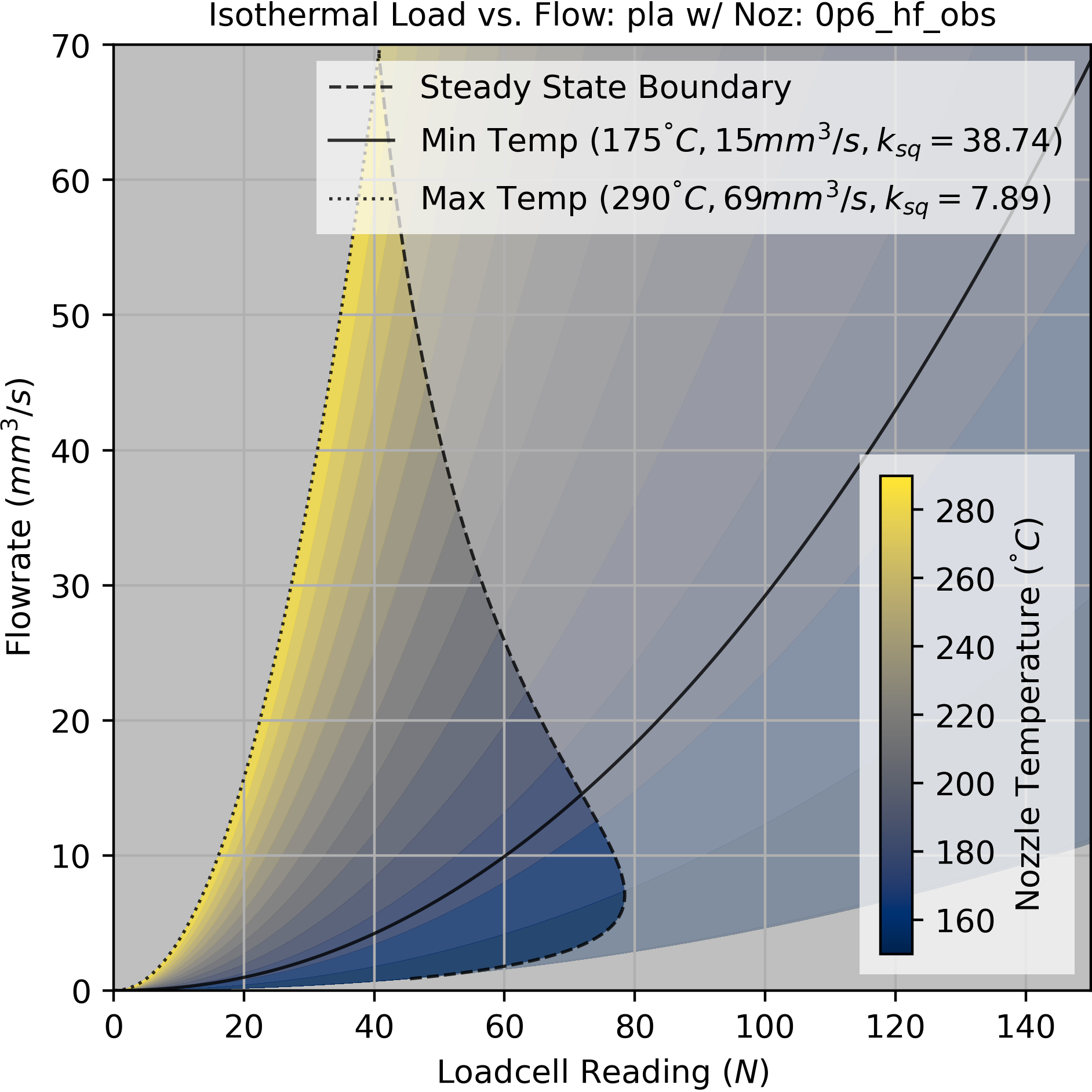
For compressibility, we fit a compression parameter \(k_{sq}\) to the filament, which estimates how much nozzle load is generated for each cubic millimeter of filament that is compressed between the extruder motor and the nozzle tip. This is effectively a springrate (units are \(N/mm^3\)). With softer filaments we need to spin up our extruder motor further in advance of our desired outflow, whereas stiffer filaments are more direct.
The pressure to flow relationship itself (at a single temperature) can be simply modelled with the function Equation 6.4, with a linear term \(a\) and power term \(b\).
\[ Q = (Fa)^b \tag{6.4}\]
In our steady-state model above, as pressure increases, steadystate flow increases but at a decaying rate - i.e. for every additional N of load, we get less return on flow (\(b < 1.0\)). However, on shorter time-scales, this is reversed: flow increases at an increasing rate for every additional N of load (\(b > 1.0\)). As already discussed, the decaying exponent in steadystate can be understood as the melt flow’s temperature dropping at larger rates (thus increasing its viscosity). On short time scales, we see polymer shear thinning[^SHEAR_THINNING], a phenomenon observed in non-newtonian fluids where increases to pressure (… shear) drop the flow’s viscosity.
6.5.4.1 Fitting Isothermal Models
For dynamics we naturally want to fit some set of ordinary differential equations (ODE)s that will predict time series behaviour of the system. Those are below in Equation Equation 6.5
\[ \begin{aligned} Q_{out} = (Fk_{lin})^{k_{pow}} \\ \dot{F} = (Q_{in} - Q_{out})k_{sq} \end{aligned} \tag{6.5}\]
The driving input to this set of ODE’s is the extruder velocity (inflow, \(Q_{in} (mm^3/s)\)) and output is the flowrate from the nozzle tip (outflow, \(Q_{out}\)), with an internal (compression) state (our loadcell reading) \(F (N)\) - this is scaled by the springrate \(k_{sq}\)
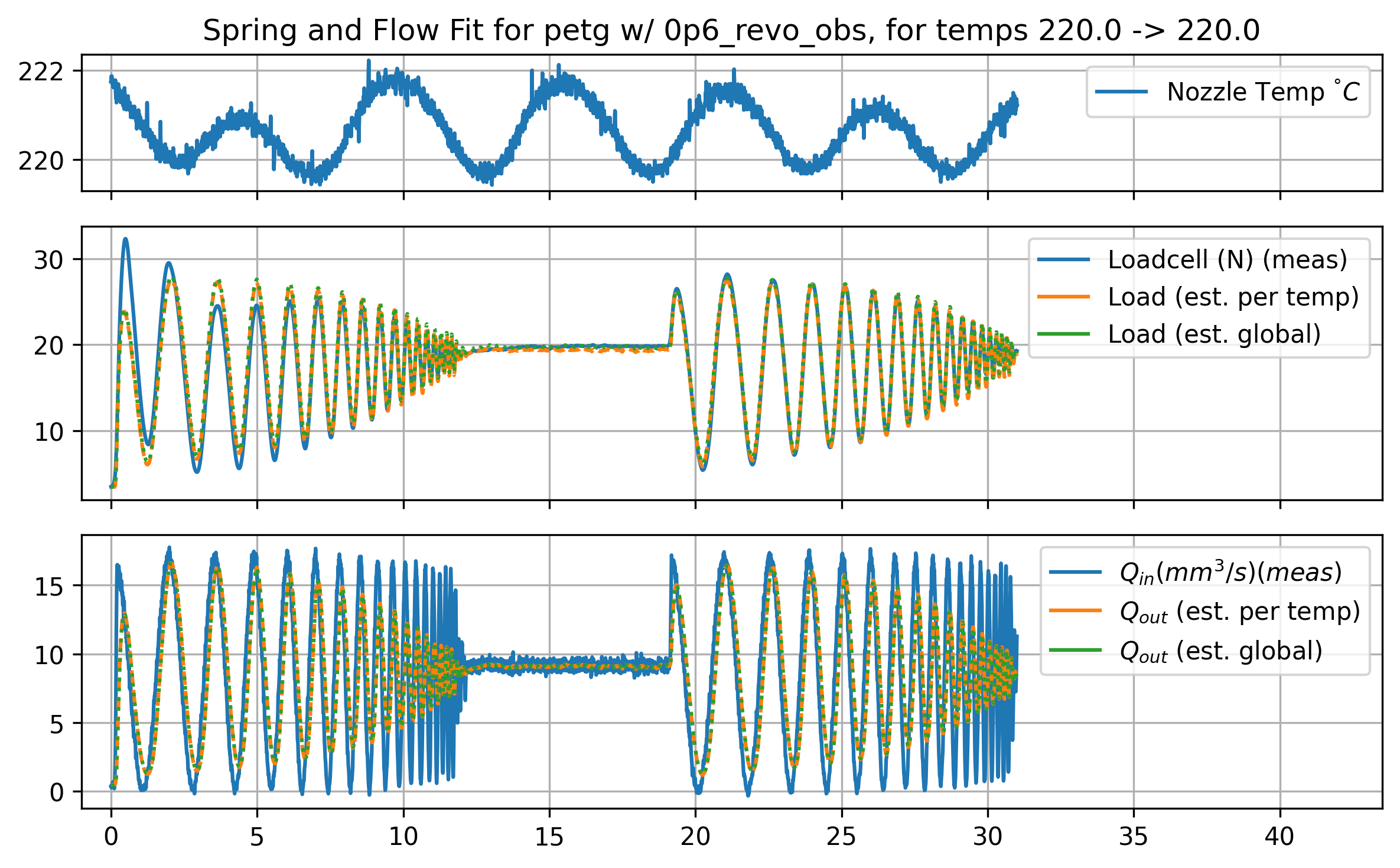
In prior work, I fit the springrate using computer vision to measure track widths (and then relate those to flowrates, using translational velocities), but I have found that we can simplify this step by adjusting the parameters of those ODEs so that our time series data for extruder load aligns with the models’ simulation. We fit to the internal state rather than the final output. This greatly simplifies the data gathering routine, allows us to extend modeling across all data gathered from the machine (rather than just in specific tests where an extruded track is clearly visible for a vision system), and fit on higher frequency data (camera frames are gathered around ~ 30Hz, but loadcell data arrives at ~1kHz).
The appropriate data to gather for a starting fit is a simple chirp signal sent into our extruder’s velocity controller. A chirp works well because it causes our model to fit the dynamic state (compression) across a range of frequencies, whereas the pressure relationship must fit consistently across the whole of the chirp. I designed a chirp that was long enough to capture enough data for the fit, but short enough that it doesn’t drive the system out of the isothermal range: i.e. it is short enough that we can assume that the melt flow does not cool substantially during the test.
6.5.4.2 Dynamics Across Temperatures
Parameters for the flow system vary across temperatures: warmer flows have smaller springrates (are more compressible), and tend to have more linear pressure-to-flow relationships. This makes intuitive sense: hot things are squishier, and more molten (less viscous) flows act more like newtonian fluids (less shear thinning).
While it would be possible to simply use the parameters we find at the temperature we choose to operate in, we can also fit a relationship between these parameters and the flow temperature. This helps us later to pick an exact temperature to operate with, and prevents us from having to fit parameters for any temperature we would like to operate with. It is also critical because in real operating conditions, the melt flow temperature is changing even when our nozzle temperature is fixed.
As we did with the steadystate model, here we fit some additional terms that modify our underling parameters across temperature.
\[ \begin{aligned} T_{norm} &= \frac{T - T_{min}}{T_{max} - T_{min}} \\ kt_{sq} &= T_{norm} \cdot a + b \\ kt_{lin} &= T_{norm} \cdot c + d \\ kt_{pow} &= T_{norm} \cdot e + f \\ \end{aligned} \tag{6.6}\]
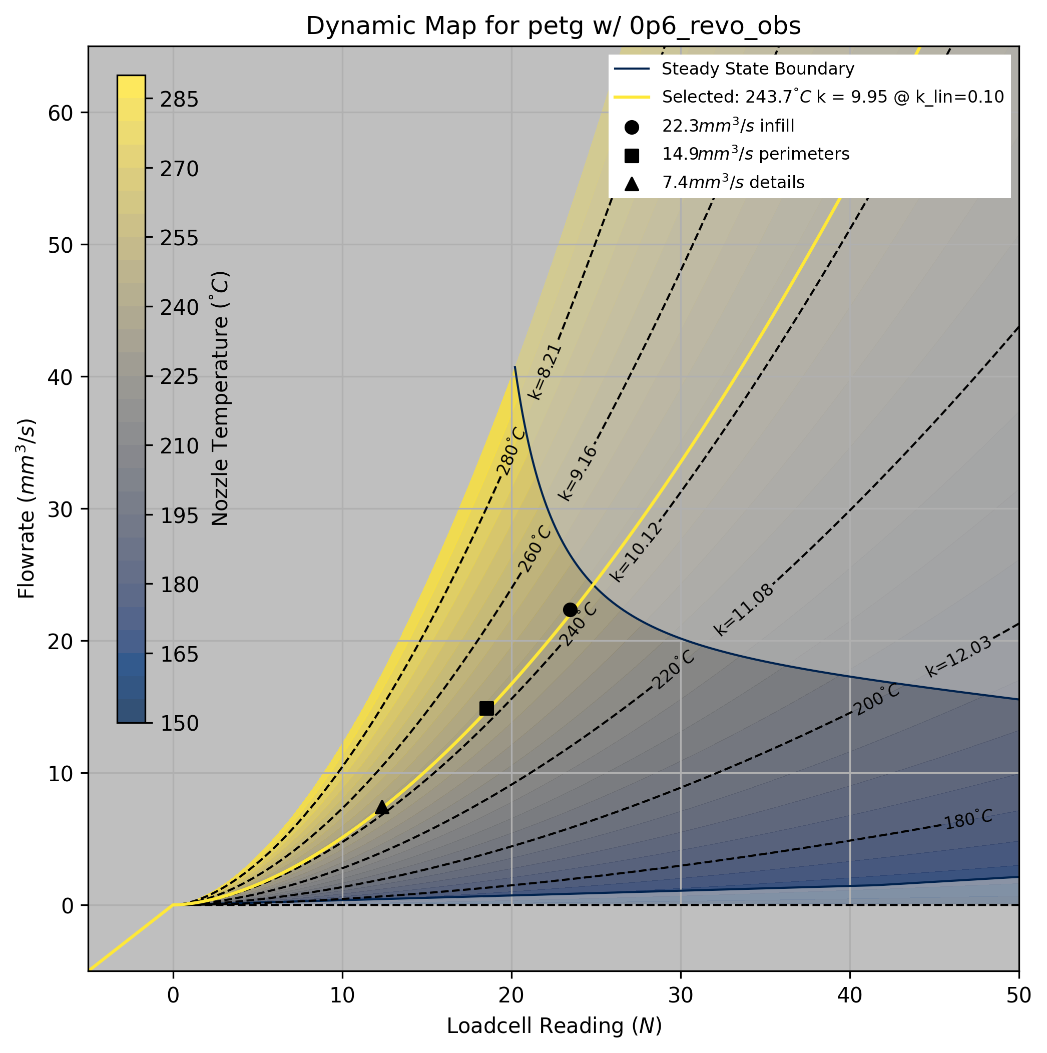
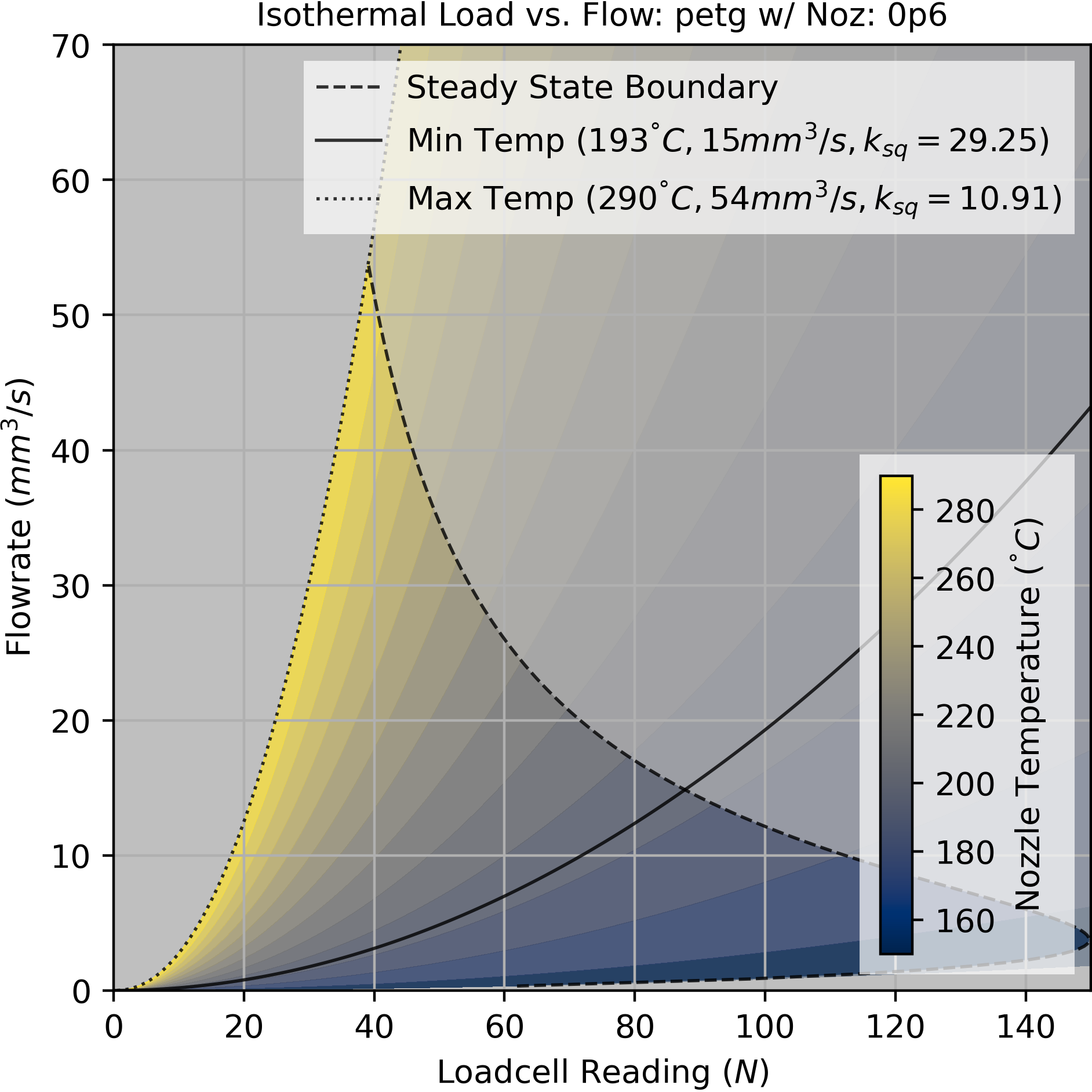
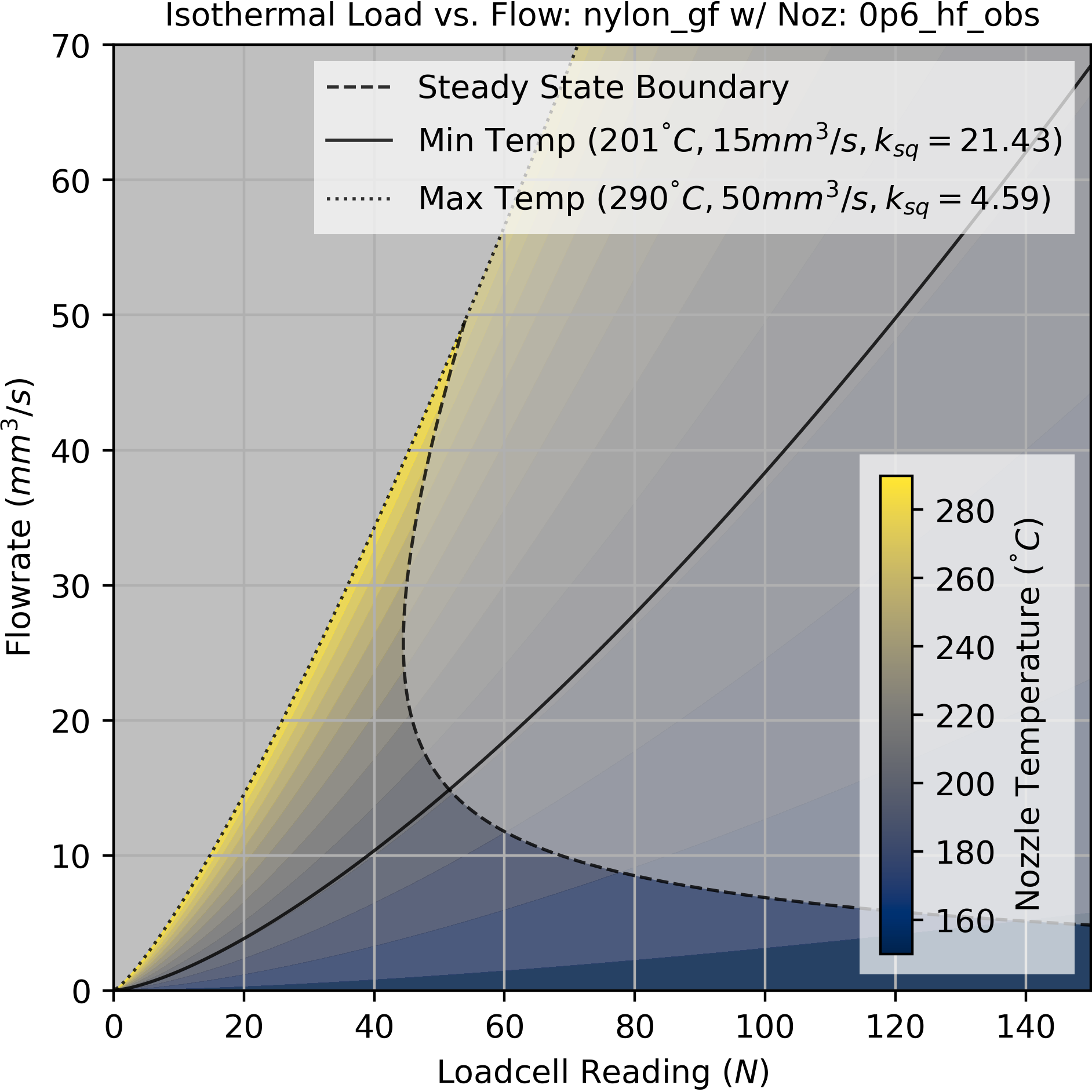
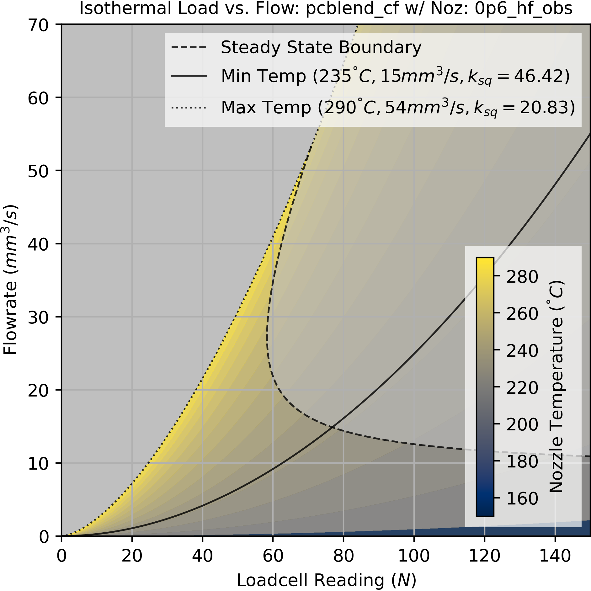
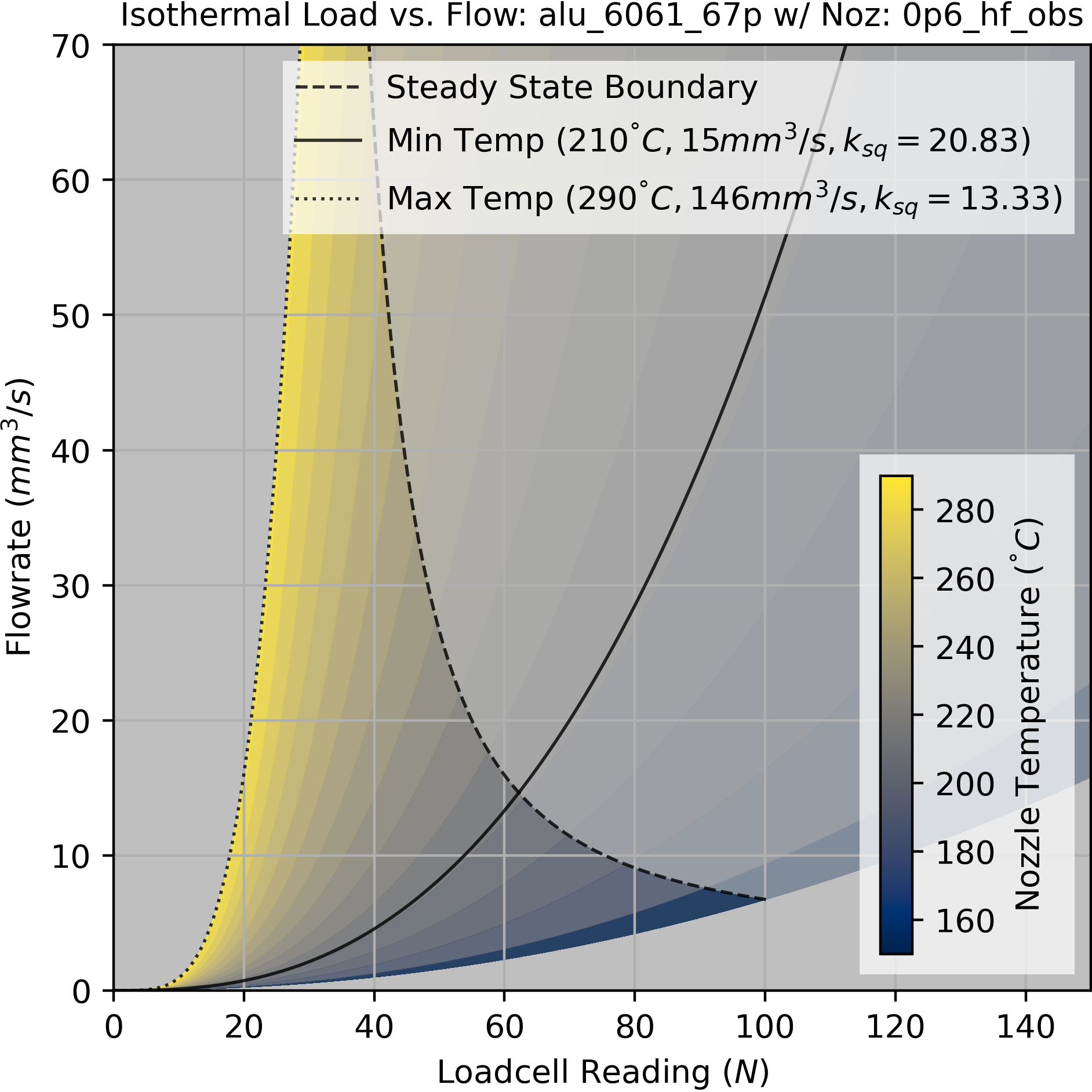
Putting this together with the steady-state boundaries discussed above, we can produce operating maps like those in Figure 6.10 above that display dynamic characteristics across temperatures, including springrates and boundaries. In Section 6.8, I will explain how we choose an operating temperature (and set of flowrates) out of this region.
6.5.5 Interploating Between Steady-State and Isothermal Operation
The tests developed here are designed to provide explicitly steady-state and isothermal data separately. In practice, the machine operates somewhere between these two ranges: long, fast sections of infill might get us close to steady-state operation, whereas slow, detailed sections of a print are close to isothermal.
Modelling this properly as a history dependent thermodynamic system would be difficult because it would add a few new internal parameters like filament conductivity, heat capacity, and might require that we accurately estimate the nozzle heater’s thermal mass, etc. Instead, we can interpolate between our steady-state and isothermal models using a measurement of the average flowrate of the filament in the melt zone.
If we compare our steady-state and isothermal models, we can see that any point in the pressure, flowrate plan returns a temperature. If we pick any point here, we have two temperatures: one from the steady-state model, and one from the isothermal model.
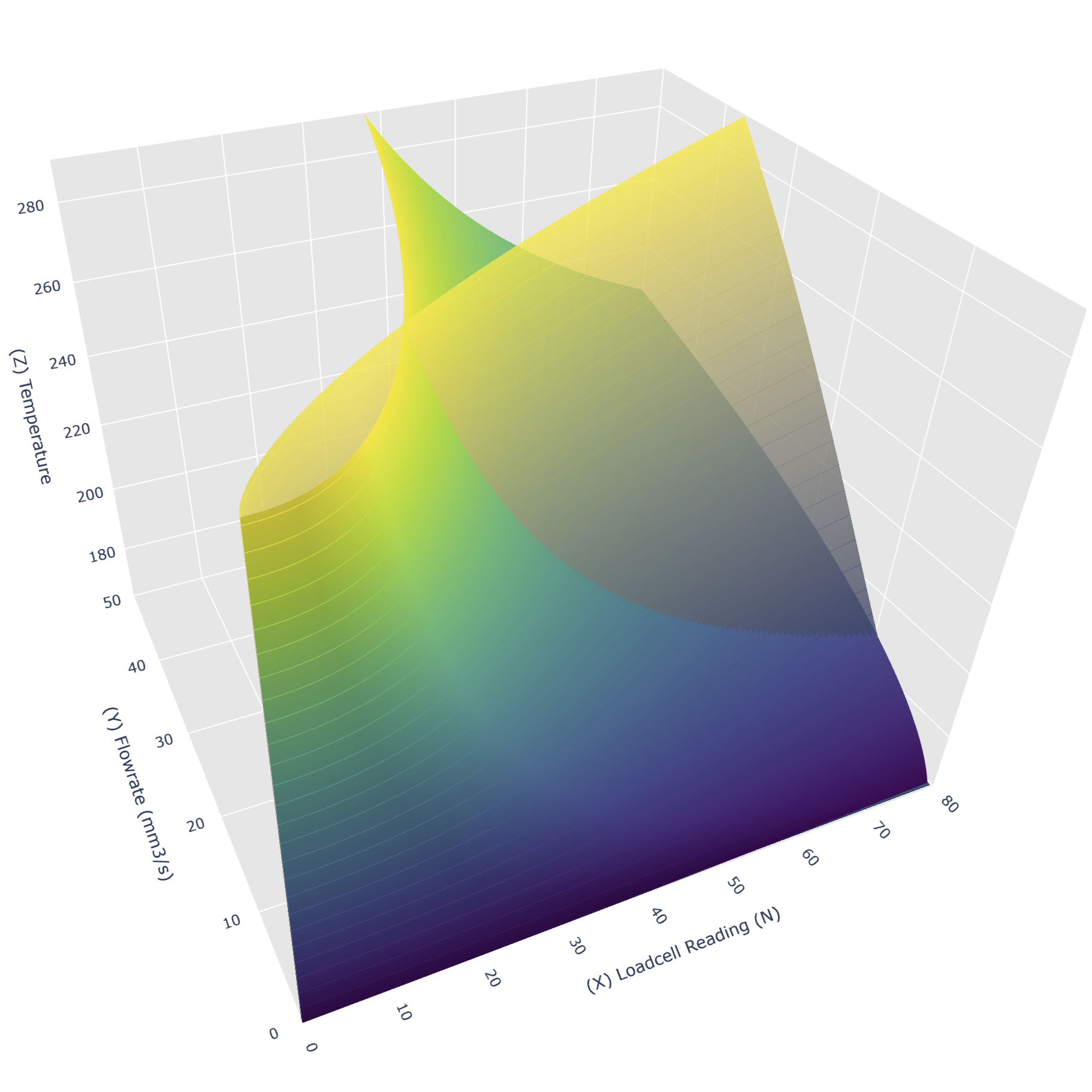
While the two models mostly overlap near the origin, the steady state model predicts larger temperatures than the isothermal model as speeds and pressures increase. If we subtract the isothermal temperature from the steady-state temperature across the operating space, we get a third map that corresponds to temperature drop of the melt flow from the nozzle temperature across the operating space.

By taking a slice of this model at the operating nozzle temperature, we can plot the expected temperature drop as a function of average flowrates at that temperature. That’s above in Figure 6.14, and is the information we will need later when we deliver these models to the machine controller.
6.6 Models for Extruder Motors
The models above are sufficient to understand the melt flow dynamics of the extruder. However, we need to drive those dynamics with our extruder motor. In fact, when we analyse printing data later in Section 6.11.2, we will see that overall print speed is often limited by the extruder motor’s ability to rapidly compress and decompress filament as the machine corners. I already covered the relevant motor physics (and our modelling strategy for the same) in Section 5.3.1. In this section, I will describe how I connect the two models with a few extra parameters, and how those parameters are fit to data.
For a refresher on motors: we have a direct relationship between stator current and torque produced by the motor. This means that motor torque is limited by current saturation. Current limits can arise for any number of reasons, but predominantly it is the motor’s ability to dissipate heat.
Most 3D Printer designs favor small extruder motors that are rated to about 0.5 Amps of continuous drive current, trading power for light-weight packaging. They overcome the resulting lack of torque by adding gear reductions, which is effective because linear filament speeds are typically low (under \(100mm/s\)). The extruders in both machines that I used here use this strategy.
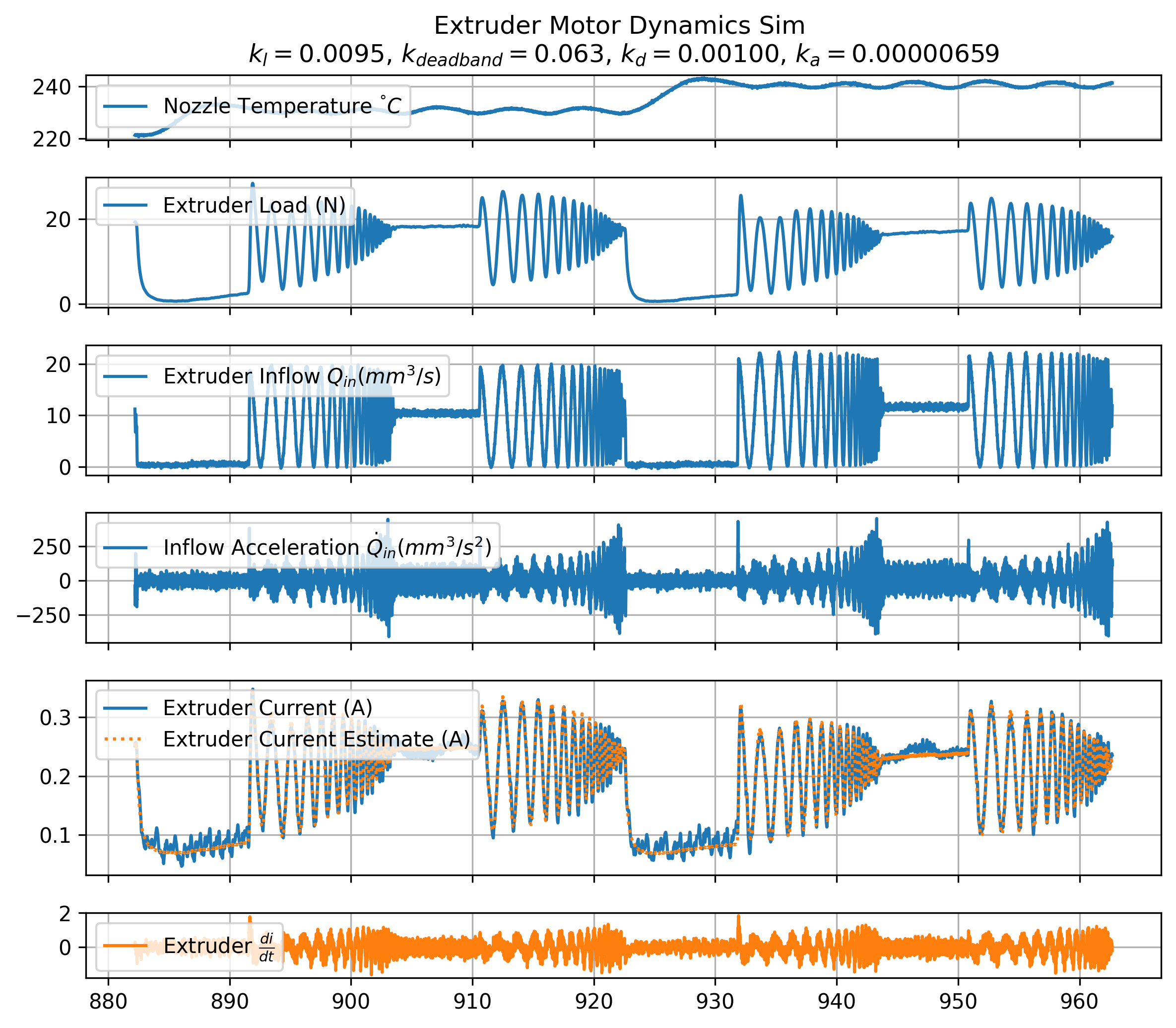
Motor dynamics are typically coupled into motion systems that have fixed mass and damping. In the extruder system, we need to add a parameter for the amount of current required to generate pressure in the nozzle. So, we use a model that predicts motor current as a function of the motor’s speed (a damping term), acceleration (inertial), and two additional parameters for pressure: a deadband (current required to generate any pressure), and a linear load factor (Amps required for every additional Newton of pressure). This is below in Equation Equation 6.7.
\[ \begin{aligned} I_{extr} = Lk_l + k_{deadband} + Q_{in}k_d + \dot{Q}_{in}k_a \\ k_l = \text{Linear Load Factor} \ (A/N) \\ k_{deadband} = \text{Load Offset} \ (N) \\ k_{d} = \text{Damping} \ (A/mm^3/s) \\ k_{a} = \text{Inertial} \ (A/mm^3/s^2) \end{aligned} \tag{6.7}\]
The damping and inertial terms are fit again in terms of the inflow - i.e. the flowrate past the extruder’s drive gears, which is exactly proportional to the extruder motor velocity (with some scalar).
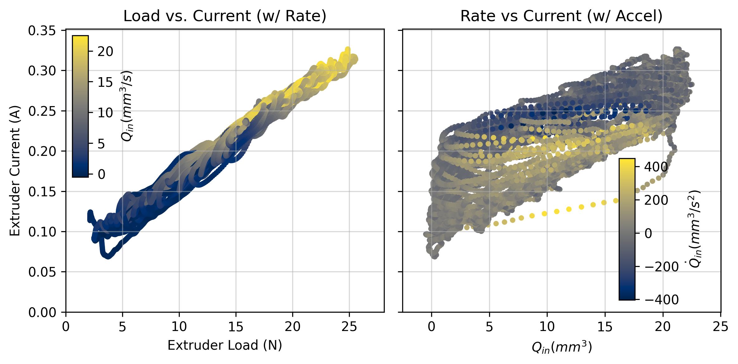
Finding the parameters for this model is simple with time series data. We typically see that our current requirement is dominated by the extruder load, with a smaller damping parameter and even smaller acceleration parameter. Even though it looks small, the acceleration parameter often becomes the critical limit during dynamic moves where optimal inflow acceleration requests can exceed \(50000mm^3/s^2\). Parameters from an example fit are called out in Figure Figure 6.16 below, where I compare time series measurements (in blue) to the model’s estimates (in orange).
6.7 Models for FFF Cooling
For our last section on modelling methods, we need to understand how the preprocessor will estimate layer cooling times. This involves one calculation to estimate volumetric heat capacity, and the development of a simple cooling model based on simple heat transfer equations.
6.7.1 Volumetric Heat Capacity
While it is difficult to develop a complete thermal model of our filament, we can at least estimate its volumetric heat capacity \((J/mm^3)\). We can make this estimate using data from our steady-state tests, where nozzle temperature decays due to losses into ambient environment and loss into the filament flow. To convert these losses into estimates of real-world units, we use our knowledge of how much power is delivered to the nozzle at any given time.
We begin with a model that estimates the change in nozzle temperature over time, below.
\[ \begin{aligned} \frac{dT}{dt} = (T_{amb} - T) k_{loss} + {Q}(T_{amb} - T) k_{flow} \end{aligned} \tag{6.8}\]
| Symbol | Units | Value |
|---|---|---|
| \(T\) | \(^\circ C\) | Temperature of Flow |
| \(T_{amb}\) | \(^\circ C\) | Ambient Temperature |
| \(Q\) | \(mm^3/s\) | Volmetric Flowrate |
| \(k_{loss}\) | \(({C/s})/{\Delta T}\) | Heat Loss to Ambient |
| \(k_{flow}\) | \(({C/s \cdot (mm^3/s)})/{\Delta T}\) | Heat Loss per unit of Flow |
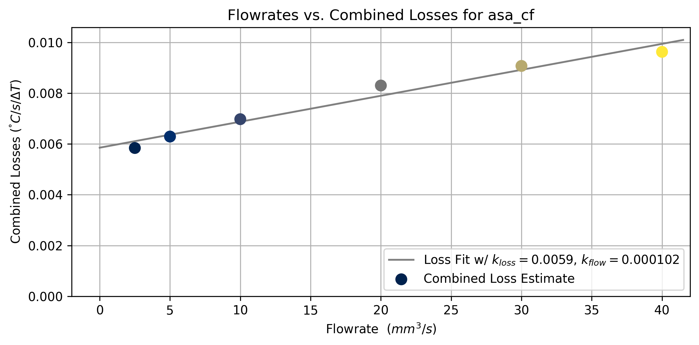
The \(\Delta T\) we use for each of these losses is from ambient temp \(T_{amb}\) to the nozzle temperature \(T\). This makes the assumption that filament heats from ambient up to the nozzle temperature before exiting the nozzle. We know that this is not always entirely true - especially at large flowrates - but it nets us an estimate that is sufficient. To fit, we first estimate the total loss across each flowrate, as in Figure 6.17.
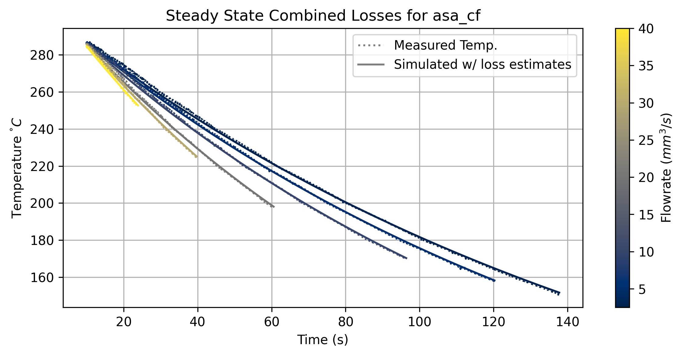
We can then plot the total losses at each flowrate. This fits a simple linear relationship, where we estimate that the offset represents our loss to ambient, and the slope represents additional loss for every unit of filament flowrate.
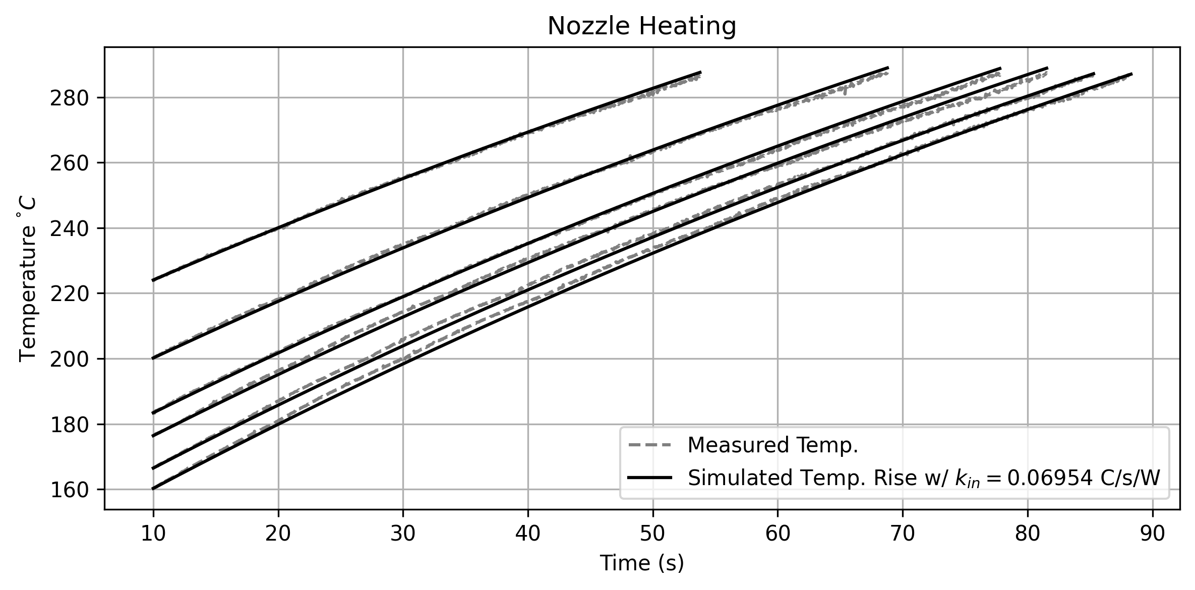
These losses are not yet power measurements. To back out a heat capacity, we need to measure the wattage required to move the nozzle temperature. For this, we can fit an additional parameter that is active when the nozzle is warming up.
\[ \begin{aligned} \frac{dT}{dt} = k_{in}W_{in} + (T_{ambient} - T) k_{loss} \end{aligned} \tag{6.9}\]
| Symbol | Units | Value |
|---|---|---|
| \(T\) | \(^\circ C\) | Temperature of Flow |
| \(T_{amb}\) | \(^\circ C\) | Ambient Temperature |
| \(k_{in}\) | \(\frac{C/s}{W}\) | Change in Temperature per Watt |
| \(k_{loss}\) | \(({C/s})/{\Delta T}\) | Heat Loss to Ambient |
We can easily measure the power into the nozzle \(W_{in}\) by measuring our heater’s resistance and the controller’s supply voltage.
We can now combine our measurements to produce an estimate for the filament’s heat capacity. If we do a little bit of units analysis (see below), we can see that the volumetric heat capacity is equal to \(k_{flow} / k_{in}\).
\[ \begin{aligned} C_v = k_{flow} (\frac{C/s \cdot (mm^3/s)}{\Delta T}) / k_{in} (\frac{C/s}{W}) \\ \frac{C/s \cdot (mm^3/s)}{\Delta T} \cdot \frac{J/s}{C/s} \\ \frac{(mm^3/s) \cdot J/s}{\Delta T} \\ \frac{J\cdot mm^3}{\Delta T} \end{aligned} \tag{6.10}\]
It is more common to measure specific heat capacity of materials (i.e. \(J/kg\)), but in our case volumetric is more useful \((J/mm^3)\). We anyways don’t have an estimate for material density (although it may be easy to generate).
Our measurements are not incredibly precise, but do put us in a reasonable ballpark for the real physical value. Polymer heat capacity is anyways nonlinear in practice (CITE), with i.e. different phases of each polymer having different heat-carrying capabilities (not to mention density changes). For our purposes an estimate is good enough.
6.7.2 Layer Cooling Time
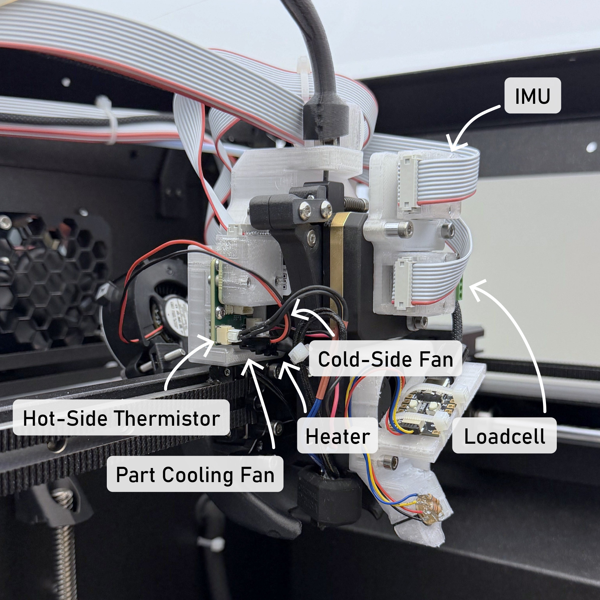
When we start printing a layer we need the previous layer to be mostly solidified. If we don’t meet this criteria, we are printing molten material on top of molten material and can quickly end up with puddles of plastic (known as slumping in FFF) instead of the components we meant to print. This is why FFF printers all include part cooling fans (PCF), which blow ambient air around the nozzle to promote layer cooling, one of which is visible in Figure 6.6. For more detail on this, and to see how we deploy these cooling models, see Section 6.8.1.
Whereas slicers use direct parameters to control part cooling (see Table 6.1), we replace those with a little bit of model building that will let us estimate a minimum layer time \((t_{min})\) - the time that we need to wait after printing a track before we can print on top of it without risk of slumping.
The rate at which the fan cools the layer is dependent on many things: the polymer’s heat capacity, its temperature, the temperature of the surrounding layers, the print geometry, and the fluid dynamics of the cooling air, the chamber temperature, etc. We will build a simple model of this that excludes those fluid dynamics, and also ignores thermal history beyond the previous layer.
For material parameters, we have the filament’s volumetric heat capacity (estimated in the section above), but we need also the filament’s conductivity \(\kappa_{fil}, \ (W/m \cdot \Delta T)\). It seems possible to estimate this value (since it factors in the filament’s ability to absorb heat from the nozzle, see Section 6.5.5), but I resort to estimates for this value instead; the typical range for our common polymers is \(0.1, 0.25.\)
We also need to estimate the effectiveness of our printer’s cooling system. This is encoded in \(h_{air}, \ (W/m^2 \cdot \Delta T)\) - energy flow out of the filament into the print chamber. An intuitive sense2 for this value is that it lies somewhere in the range \(10, 100\), and fan-driven cooling rates are relatively well tabulated in engineering references. Luckily this value is tied to the machine (not the material), so we can tune it over time.
We use the materials’ conductivity to estimate the cooling rate into the layer below \(h_{layer}, (\ W/m^2 \cdot \Delta T)\) - this is a function of the layer height, and is further shimmed by an estimate of the layer to layer contact \((l_{iface})\), giving us \(h_{layer} = (\kappa_{fil} / H) \cdot l_{iface}\).
Finally we need to pick a target cooling temperature \(T_{targ}\) - we want this to represent the temperature where our layer is going to be solidified enough to support subsequent layer geometry. This is a real decision variable: for intricate parts we want our previous layers to be relatively cold. With large, blocky prints we can get away with a bigger value here. I tune this relative to the material’s zero flow temperature (from Section 6.5.3). My reasoning is that, when the material is cold enough that it cannot be extruded, it will be relatively stiff. This is exposed as one of the preprocessor inputs as a \(\Delta T\) such that \(T_{targ} = T_{min} - T_{cool}\)
| Symbol | Value | Units | Source |
|---|---|---|---|
| \(H\) | Layer height | \(mm\) | Part Geo. |
| \(l_{iface}\) | Layer interface proportion | 0-1.0 | Part Geo. |
| \(\kappa_{fil}\) | Filament conductivity | \(W/m \cdot \Delta T\) | Estimated |
| \(C_{fil}\) | Filament heat capacity | \(J/m^3 \cdot \Delta T\) | Model Fit |
| \(T_{noz}\) | Nozzle temperature | \(^\circ C\) | Direct Measurement |
| \(T_{targ}\) | Cooling target temperature | \(^\circ C\) | From Flow Models |
| \(T_{amb}\) | Ambient temperature | \(^\circ C\) | Known |
| \(h_{air}\) | Heat transfer to air | \(W/m^2 \cdot \Delta T\) | Estimated |
| \(h_{layer}\) | Heat transfer to layer below | \(W/m^2 \cdot \Delta T\) | Via \(fil_k\) |
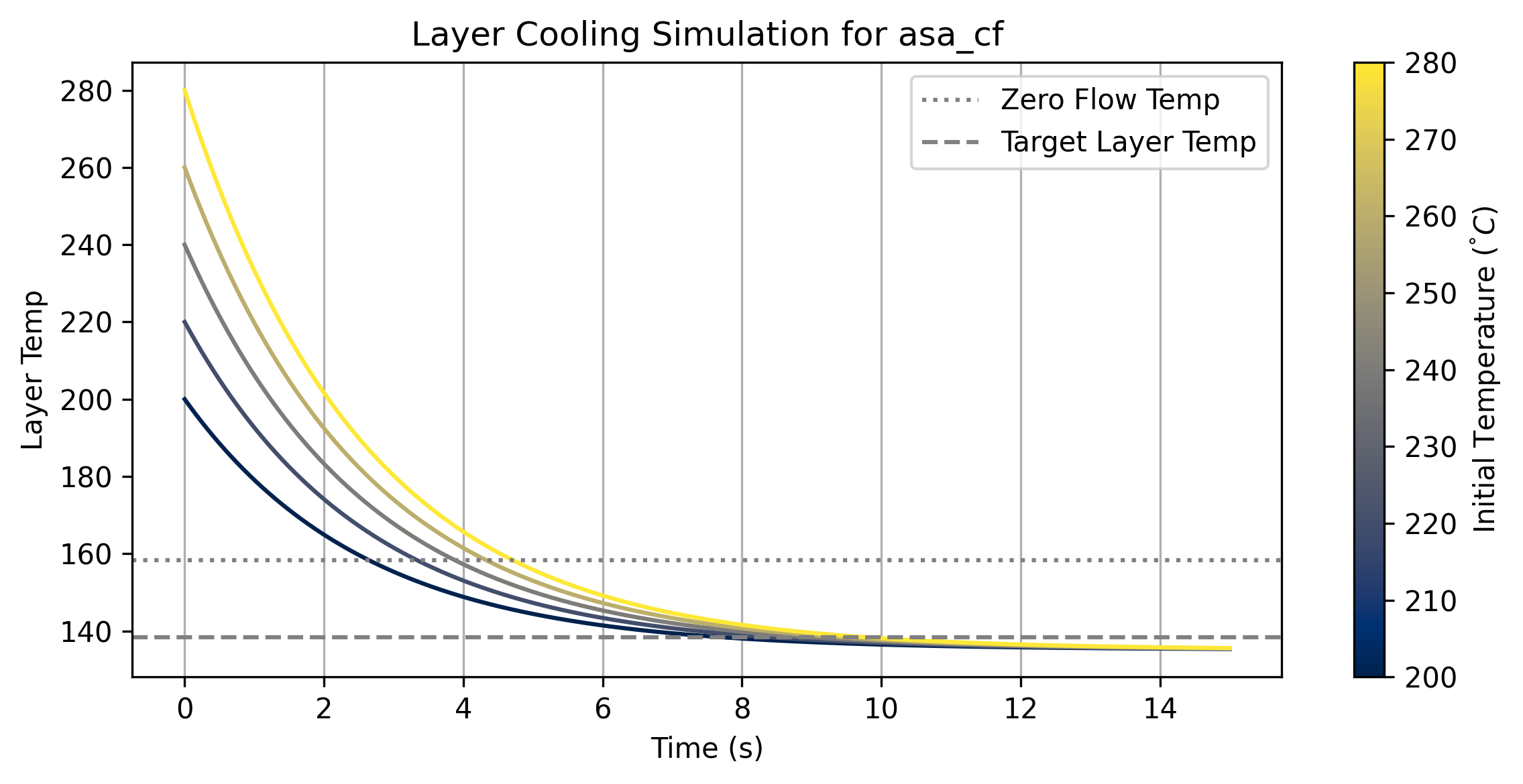
We can work out a cooling time constant \((\tau)\) using Equation 6.11, and an equilibrium temperature \((T_{eq})\) using Equation 6.12. Finally, we use these to calculate the layer cooling time \((t_{min})\) with Equation 6.14.
\[ \begin{aligned} \tau = (C_{fil}) / (h_{air} + h_{layer}) \end{aligned} \tag{6.11}\]
\[ \begin{aligned} T_{eq} = \frac{(h_{air} \cdot T_{amb} + h_{layer} \cdot T_{targ})}{(h_{air} + h_{layer})} \end{aligned} \tag{6.12}\]
\[ \begin{aligned} h_{layer} = (\kappa_{fil} / H) \cdot l_{iface} \end{aligned} \tag{6.13}\]
\[ \begin{aligned} t_{min} = -\tau \cdot log((T_{targ} - T_{eq})/(T_{noz} - T_{eq})) \end{aligned} \tag{6.14}\]
This model is approximate. For example our equilibrium temperature calculation assumes that the previous layer’s temperature is a boundary condition, when of course it actually continues cooling into the layer below it as time progresses. This means that we probably over estimate layer cooling times, especially in large prints. Our model could be extended across each layer, but we would need to develop a much more complex (and probably geometric) solver for this - the approximation works well enough especially considering that we are already estimating \(h_{air}\) and the filament’s conductivity.
6.8 High Level FFF Planning
Now that we have seen the modelling methods, we can proceed to look at the preprocessor step in the workflow. This is where we combine our part file (geometry) and models with heuristics, to select high level operating parameters. First I will show how we select a time-optimal nozzle temperature based on cooling and flow models, and then how we develop and apply motion and extruder heuristics.
6.8.1 Time-Optimal Nozzle Temperature Selection
- Nozzle temperature is probably the single most important parameter in FFF 3D Printing.
- Models let us operate the printer in any of a range of viable temperatures,
- Here, we will pick a particular temperature using our cooling and flow simulations, and a simple optimization over temperatures to minimize total print time.
- Hot nozzles give us fast flows, but increase layer cooling time.
- Small parts tend towards colder flows, because layer cooling time dominates total time. Vise versa for large parts.
![]()
![]()
6.8.1.1 Nozzle Temperature Lower Bound
First, we want to pick a lower bound for nozzle temperature. The simplest metric for this is to select the coldest temperature that makes a minimum flowrate possible.
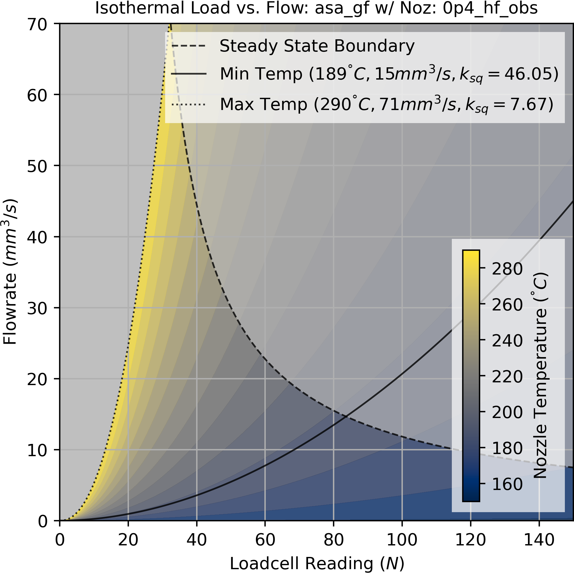
The minimum flowrate is a selected heuristic, for example I set this to \(15mm^3/s\) in the prints in this section. The minimum temperature is found by intersecting that flowrate with the steady state boundary curve (shown above), which is parameterized as a function of temperature.
6.8.1.2 Selecting Flowrates using Models and Heuristics
When we pick a temperature, we also select target flowrates for three different types of segments (infill, perimeters, and details) using models and heuristics. For each segment type, we pick a scalar in \(0-1.0\). At any temperature, we take the pressure at that temperature’s maximum flowrate as \(1.0\) and then select target pressures according to those scalar values.
This process nets us a maximum translational rate per segment, by dividing the segment’s width (which is effectively \(mm^3/mm\)) by the selected flowrate for that segment type. This step encodes both flow heuristics (flow is tidier and more linear at lower pressures) and motion heuristics: we care more about the quality of our part’s perimeters and details than we do about its infill. By selecting larger pressure scalars for infill, we allow the machine to use more translational velocity but that velocity is carefully calibrated with respect to flow. Accelerations are also model / heuristically tuned using current scalars, as I discuss in Section 6.8.2.1.
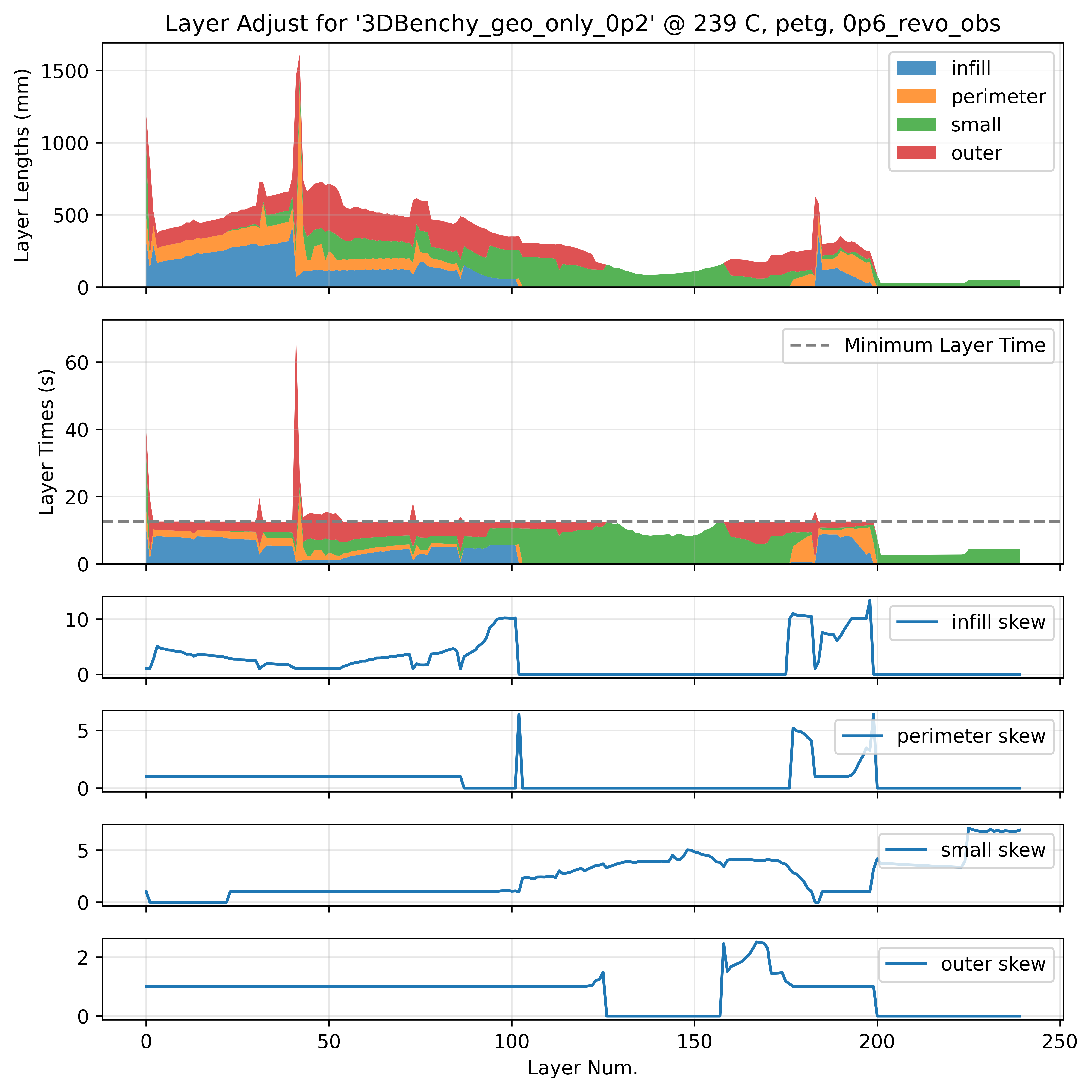
6.8.1.3 Adjusting Segment \(V_{max}\) for Minimum Layer Times
Given a nozzle temperature and it’s velocity selections described above, we can estimate the total layer time for any layer in the part at any temperature. To enforce minimum layer times, we skew velocities within each layer such that the layers total time increases. However, we prefer to skew velocities in segments that are less critical to our overall dimensions and appearances, i.e. the infill is modified first, if this does not suffice we move to the perimeters, and if this is still not enough we modify the external perimeters. This insight comes from Prusa Research’s note on the topic (Prusa Research 2024): polymer tracks extruded at higher speeds / pressures have slightly different visual properties (more matte) than those printed at lower speeds (which tend to be glossier). They also have different rates of die swell. To reduce these effects, we try to avoid skewing external perimeters unless it is truly necessary for the target lap time. Finally, we have a global limit to the skew, such that no segments have a translational velocity of less than \(10mm/s\).
6.8.1.4 Optimal Nozzle Temperature for Minimum Print Times
So by now we can pick a viable temperature range from some minimum up to the nozzle’s maximum, and then at any temperature we can select flowrates for each segment type, and calculate and then enforce a minimum layer time. Having done all of that work, we can easily pick a nozzle temperature that will give us the minimum total print time.
This optimization turns out to be exceptionally simple and intuitive. In smaller parts, total print time tends to be dominated by the minimum layer time and so colder nozzle temperatures (less cooling) are preferred. As parts increase in size, print time is dominated more by the flowrate / time to actually deposit the layer - so we want to increase the temperature to increase these flowrates.
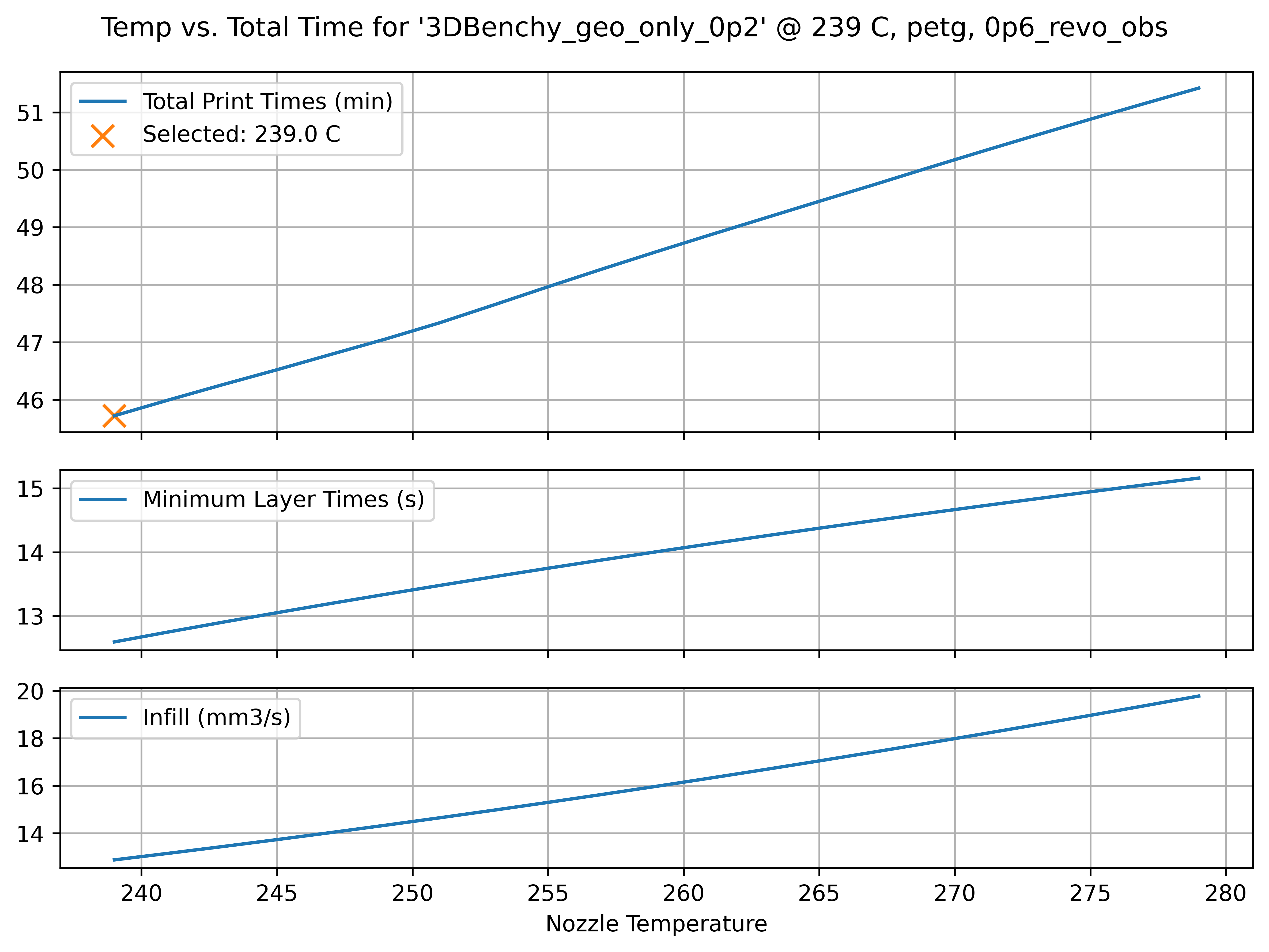
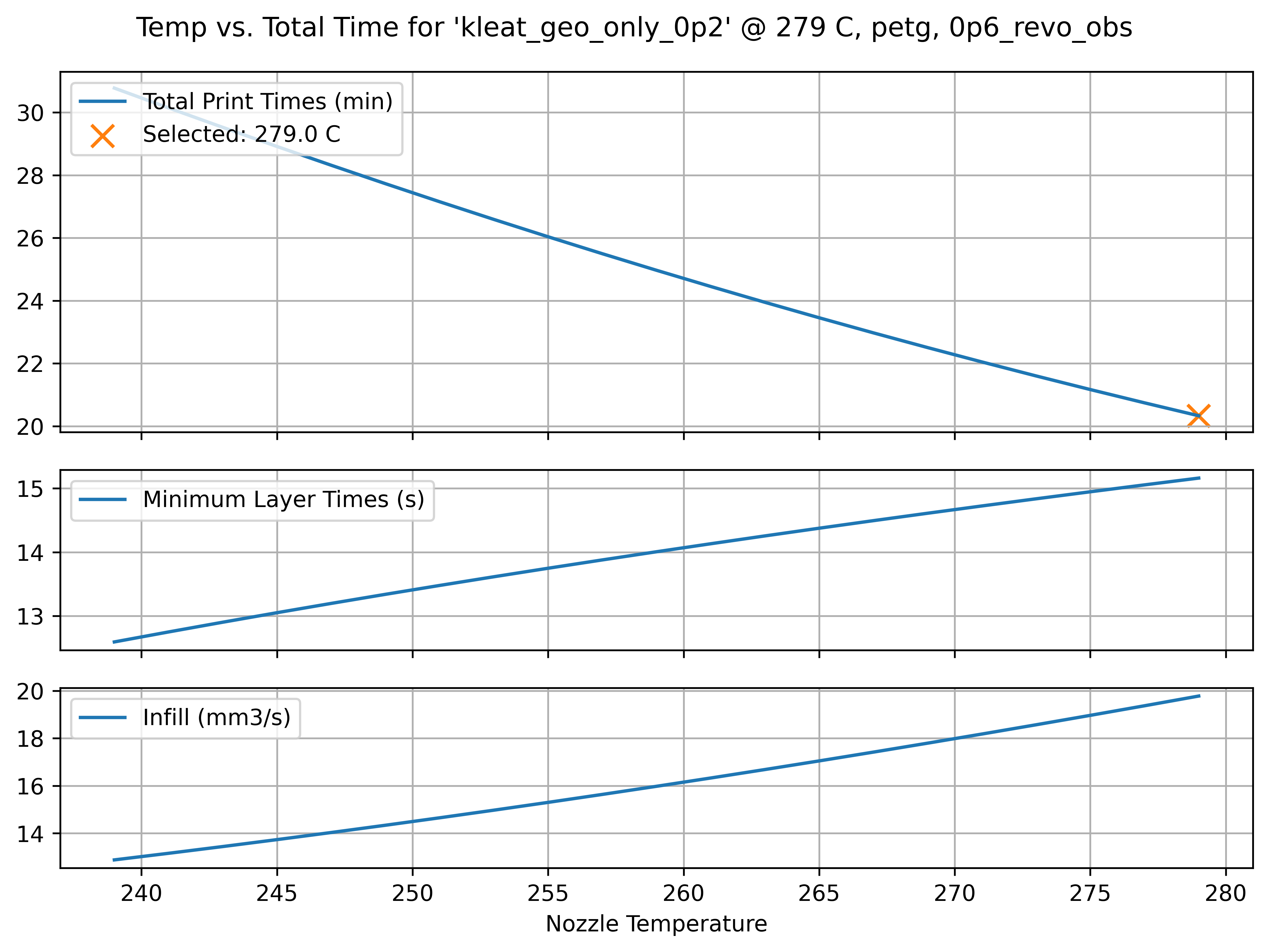
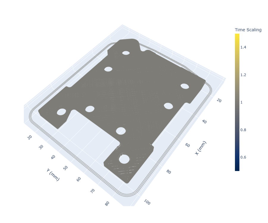
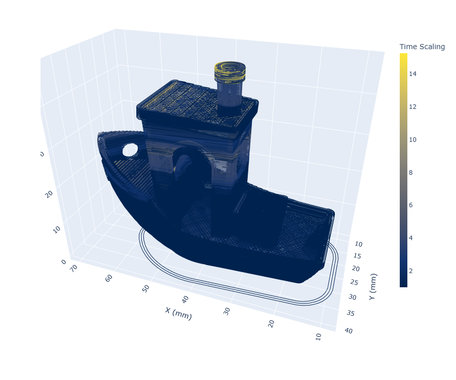
There is a crossover print size that depends on our cooling models, i.e. in the RheoPrinter with PETG (and a 0.6mm Nozzle) I found that prints about Benchy sized (60x30mm) clearly favour cold flows, whereas even slightly larger prints (90x70mm) clearly favour maximally hot flows (Figure 6.23). Parts in between exhibit a clear optimum temperature somewhere between our minimum and maximum temperatures. In these cases, flowrates and layer times increase together and balance such that the average layer time naturally meets the minimum layer time (Figure 6.24). If we increase our estimate of the printer’s cooling capability, the crossover size gets smaller (and vice versa). For polymers where temperature increases don’t lead to exceptional gains in flow, colder temperatures overall are preferred, etc.
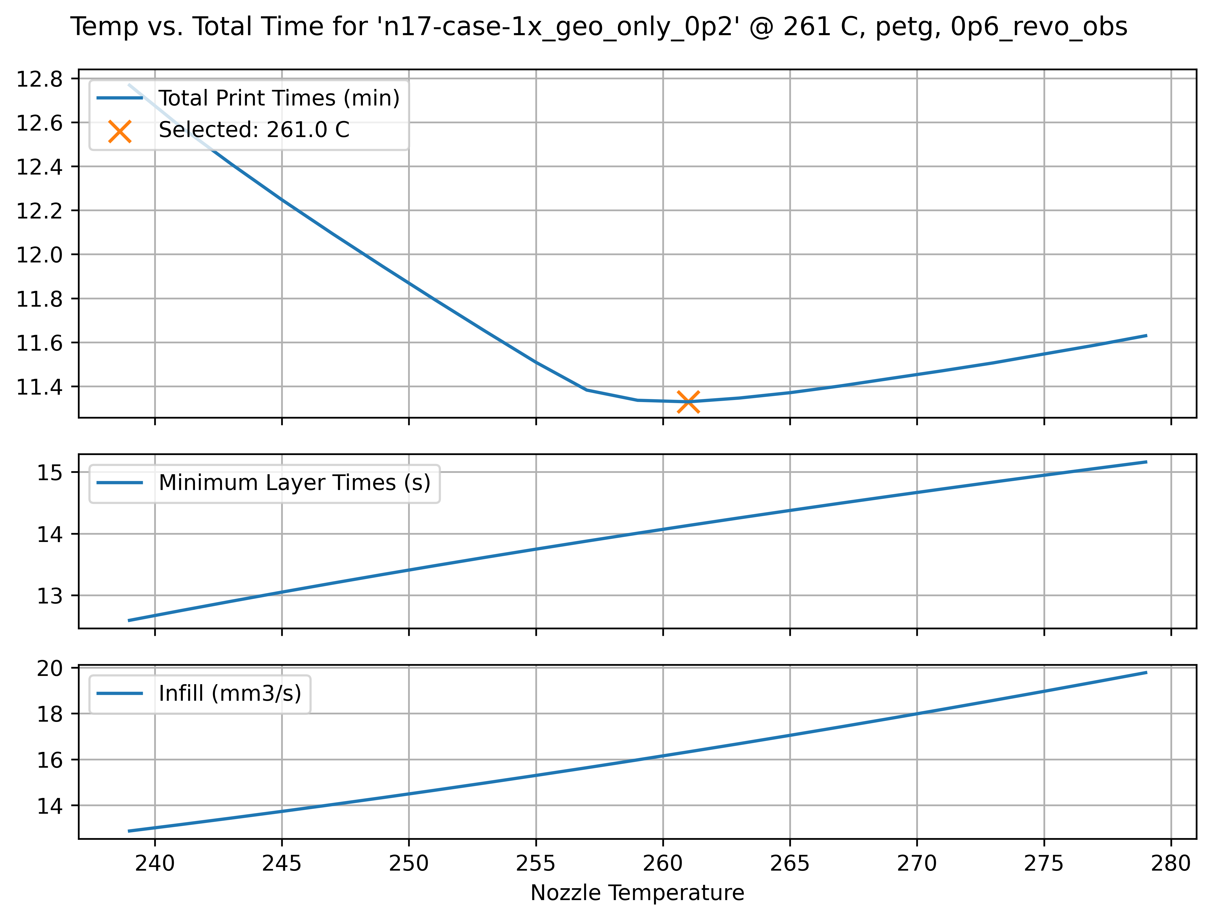
I had always thought that printers were over-optimized for producing small, detailed parts. The 3DBenchy is the de-facto parameter tuning object partially because it encapsulates lots of different features but also because it prints relatively quickly which decreases the loop time for tuning iterations. However, we typically print larger beds with i.e. multiple small parts or larger single parts. This basically means that print which have been hand tuned tend to favour colder temperatures overall, even though there are huge speed gains to be had by increasing the nozzle temperature, i.e. we can select a very hot flow for the larger part in Figure 6.23 (second row) that decreases the total print time from 30 minutes to 20 minutes. In the case of this work, because we develop print parameters over the entire range of viable temperatures, we can more flexibly adjust that single parameter and let our models and “meta heuristics” dial out the rest of the knobs.
6.8.2 Applying Motion Heuristics
6.8.2.1 Speed at Perimeters and Small Features
As I mentioned above, we typically care more about the quality of our print’s outer tracks (perimeters) than its infill. We also know (heuristics!) that when a motion system is operating near its limits, it will generally move with less grace. This is an incredibly imprecise statement, but we are talking about heuristics here.
To trade off on this front, the state of the art workflow lets us tune translational rates (across segment types) directly. As I’ve discussed, this presents the issue of scaling flowrates alongside translational rates. It also does not show us how close to the motion system’s actual limits those rate selections are, we must guess and check. Our strategy here uses flow models and normalized pressure targets for the same task (Section 6.8.1.2).
We also want to scale accelerations. We have an excellent basis for this in the motion models of our machine, whose fundamental limits come from current saturations in the actuators. If we scale the maximum current that the machine is allowed to deploy, we scale its acceleration. Here we are using the same strategy as in the flowrate selection: using a scalar to de-tune the system from its absolute limits.
I additionally scale the actuators’ deployment of \(\frac{dI}{dt},\) rate of change of current. This value corresponds to jerk, the third derivative of position (and first of acceleration). Reducing jerk further smooths motion, and reduces the frequency of the disturbances that the actuators will send into the mechanical system.
In all, we have eight heuristics that we apply at this level, all listed in Table 6.5 under Current Scalars and Current Slew Rate Scalars. The preprocessor applies those on a per-segment basis to the geometry, which can be seen in Table 6.3.
6.8.2.2 First Layer Speed
FFF veterans know well that the quality of a print’s first layer is critical. In fact, there is an entire subreddit deciated to images of high quality first layers3.
The main difference between this layer and the rest is that it must adhere to the printer’s bed, rather than to itself. Depending on how readily our print material sticks to our bed material, we want to reduce the speed at this layer so that adhesion is sure to work. It is almost always the case that bed adhesion is much worse than layer-to-layer adhesion: bed are engineered to stick well but not so well as to prevent us from retrieving our prints! To ameliorate this, first layers are normally printed at ~ 20% of the “normal” speeds. Lowering the speed gives the polymer more time to bond to the bed, and reduces vibrations or other errors that arise from translating around too fast.
While it should be possible to build a model for bed (and inter-layer) adhesion, I have not been able to do this yet. So, we stick with heuristics: first layer speeds are capped at some direct value, which can be calculated as 10% of the maximum flowrate given by our extruder model, or set directly as a maximum traversal rate in mm/sec.
6.9 Real-Time FFF Planning
I have mentioned constrained optimization in a number of places. In the previous section, we looked at how models can be used to select operating parameters for our 3D Printer by selecting operating regimes within a set of constraints (models that describe flow), and then optimizing one of the free parameters (nozzle temperatures) using models for cooling.
In the final step of our workflow, we need to actually operate the machine’s hardware in real-time to fabricate the part. This is where our lower level constraints and models become important. The run file we generated in the preprocessor contains line segments, each with a maximum velocity (set using flow models) and actuator current deployment limits (set as a normalized amount of those actuators’ total available current).
The machine cannot change velocities or flowrates instantaneously. The motion system has natural limits to velocity, acceleration, and jerk and the extruder system has limits to flowrate, flow acceleration and deceleration, and (since the extruder motor has limited \(\frac{dI}{dt}\)) even to flow jerk.
This step requires a velocity planner, which I have already discussed in Section 5.6; it explicitly solves this step as a constrained optimization problem. In this section, I extend that planner to account not only for motion dynamics, but for flow and extruder dynamics as well.
6.9.1 Optimization Formulation
The solver’s formulation and framework is explained in Section 5.6. This section describes how it is extended to include printer flow dynamics.
- The run file is segmented into \(0.05mm\) line segments, each has:
- \(v_{max} (mm/s)\)
- \(Q_{targ} (mm^3/mm)\)
- \(I_{max} (A)\)
- \(\frac{dI}{dt}_{max} (A/s)\)
- As in Section 5.6, the solver selects \(V(s)\) - velocity for each spatial segment.
- \(v(s)\) is expanded through kinematic, actuator, and flow models to generate \(I(s)\) for each actuator, \(\dot{e}(t), \ddot{e}(t),\) etc,
- A cost function penalizes over-use of current and rewards minimal window time,
- Solutions are posted to hardware via OSAP / Pipes / MAXL
- Data are collected via the same.
6.9.2 Calculating Extruder Constraints
6.9.2.1 Melt Flow Temperature Calculation
- Each \(v(s)\) is equal to some \(\Delta t\)
- Outflow \(Q_{out}(s)\) is given by \(v(s) (mm/s)\) and \(Q_{targ}(s) (mm^3/mm)\)
- I develop an associative scan that computes (in parallel) the \(Q_{out,avg}(s)\)
- We use our model from Section 6.5.5 @ the selected nozzle temperature to calculate the actual melt flow temperature at any \(s,\) \(T_{q}\)
6.9.2.2 Extruder Current Calculation
- For each point, we get required nozzle pressure using flow model \(P(s) = f(T_{q}(s), Q_{out}(s))\)
- Required volume of compressed filament from spring model, \(V_{sq}(s) = P(s) / k_{sq}(T)\)
- Each time-step has a \(\Delta V_{sq} = V_{sq, k} - V_{sq, k-1}\)
- Add to this the outgoing volume, \(\Delta V_{sq, req} = \Delta V_{sq} + Q\)
- Extruder Inflow \(Q_{in} = \Delta V_{sq, req} / \Delta t\)
- Extruder Current Requirement with Section 6.6, \(I_{e, req}(s) = f(P(s), Q_{in}(s), \dot{Q}_{in}(s))\)
6.9.3 The Cost Function
- \(v(s)\) are transformed (as described above) into:
- Extruder inflow and inflow acceleration \(Q_{in}(s), \dot{Q}_{in}(s)\)
- Extruder current requirements \(I_{e, req}(s)\)
- Extruder current slew requirements \(\frac{dI}{dt}_{e, req}(s)\)
- Motion current requirements \(I_{abz, req}(s)\) (5.6.1.2)
- Motion current slew requirements \(\frac{dI}{dt}_{abz, req}(s)\) (5.6.1.2)
- Values in these series’ are compared to maxima, (5.6.1.4)
- Each actuator has \(I_{max} = f(V_{actu})\) motor model (electrical half)
- Each is scaled by heuristic!
- Costs for exceeding limits is large, but smooth.
- Final cost item: total time for the solution window.
6.9.4 Connecting the Solver to Hardware
The solver works in space, velocity domain, aka phase space in motion control literature. Each solve cycle, we interpolate from phase to time domain to generate series of (fixed interval) control point outputs.
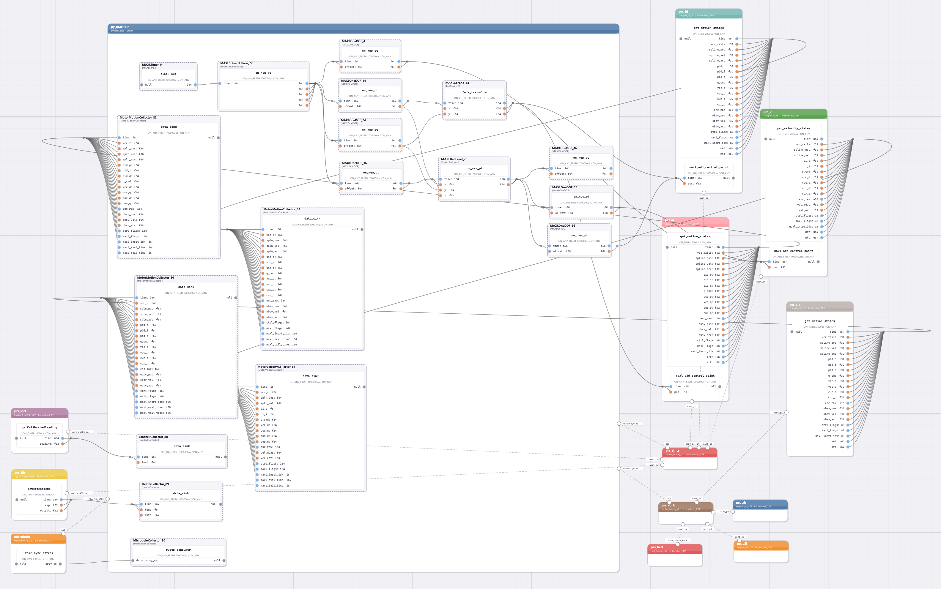
As I discussed in Section 5.6.2, the solver is instantiated as a Pipes (Section 3.2) block via an interface class that relays data into- and out-of pipes using sockets. It is connected as a MAXL (Section 3.3) component, and solution components emerge as spline control points, metered by a maxl timer block. Those go to actuators, which each runs low-level PID controls - for position (ABZ) and velocity (PI, for E). Data from motors and sensors are piped back into data collector classes, which store timestamps and samples.
6.10 Evaluating Model-Based FFF
In this section I evaluate the printing workflow developed above by:
- making one-to-one comparisons of our system against expertly developed parameter “presets” for a range of material, evaluating on print speed and quality
- demonstrating how our system reduces the size of the parameter space that needs to be tuned “by hand”
- demonstrating that our system can print new, rare and renewable materials for which expertly tuned presets are unavailable,
- demonstrating how model based control can generate data and feedback for machine users and designers that are unavailable on conventional systems
So, armed with this comparison tool, I chose a range of filaments to develop models and test prints for. I chose a set that includes the incredibly common “defaults” like PLA and PETG (which are useful because they are well understood), as well as filled versions of the same, because it is often difficult to ascertain exactly what these blends are and our system can operate well even with that uncertainty. I also included some high performance materials that are classically difficult to print like Nylon and PolyCarbonate-ABS blends (and both with glass or carbon fill), since these are excellent engineering materials and I was curious to see if our system could manage to learn how to print with them. Finally I included natural materials that are interesting for their renewable properties. For example NuTan is a material developed by a CBA Collaborator (Kubusova and Kral 2023) (which is not commercially available yet as a filament), but is made from organic feedstocks. There are no presets available for NuTan, which could limit it’s real-world adoption, so I wanted to see if we could automatically develop these. Finally I included an Aluminum Fill material because I was interested to see a thermodynamic outlier; it’s conductivity and heat capacity should me much larger than other polymers.
I also printed parts using three different nozzles; a 0.4mm brass nozzle (which is most common), and two 0.6mm nozzles. One of these is brass, and the other has a copper core, hardened steel tip, and more complex internal geometry that is designed to improve flowrates. It is also finished with a high hardness coating (“E3D Obxidian Nozzles” 2022) in order to resist abrasion from filled filaments. Along this axis, I show how our flow models adapt not only to changes in material but also to changes in nozzles.
I’ve organized these by filament, roughly in order of most- to least-common. I present a flow model and at least one test part per filament, and (where they are available) compare those to prints on an unmodified Prusa Core One. In all cases, I use geometry generated by Prusa Slicer (“Prusa Slicer” 2025) (version 2.9.2) using the 0.2mm Speed preset, with 50% infill. The workflow is shown in Figure 6.3 above.
6.10.1 Printing with the Model-Based FFF Workflow
6.10.1.1 PLA, 0.6mm Brass Nozzle
(Polylactic Acid)
![]()
![]()
![]()
![]()
6.10.1.2 PETG, 0.6mm Brass Nozzle
(Polyethylene Terephthalate Glycol)
![]()
![]()
6.10.1.3 PETG (with Carbon Fiber Fill), 0.4mm High Flow Nozzle
![]()
![]()
![]()
![]()

![]()
![]()
6.10.1.4 ASA (with Glass Fill), 0.4mm High Flow Nozzle
![]()
![]()
![]()
![]()
6.10.1.5 Nylon (with Glass Fill), 0.6mm High Flow Nozzle
![]()
![]()

![]()
![]()
![]()
![]()
6.10.1.6 PCBlend (with Carbon Fiber), 0.6mm High Flow Nozzle
(Polycarbonate + ABS)
![]()
![]()

![]()
![]()
![]()
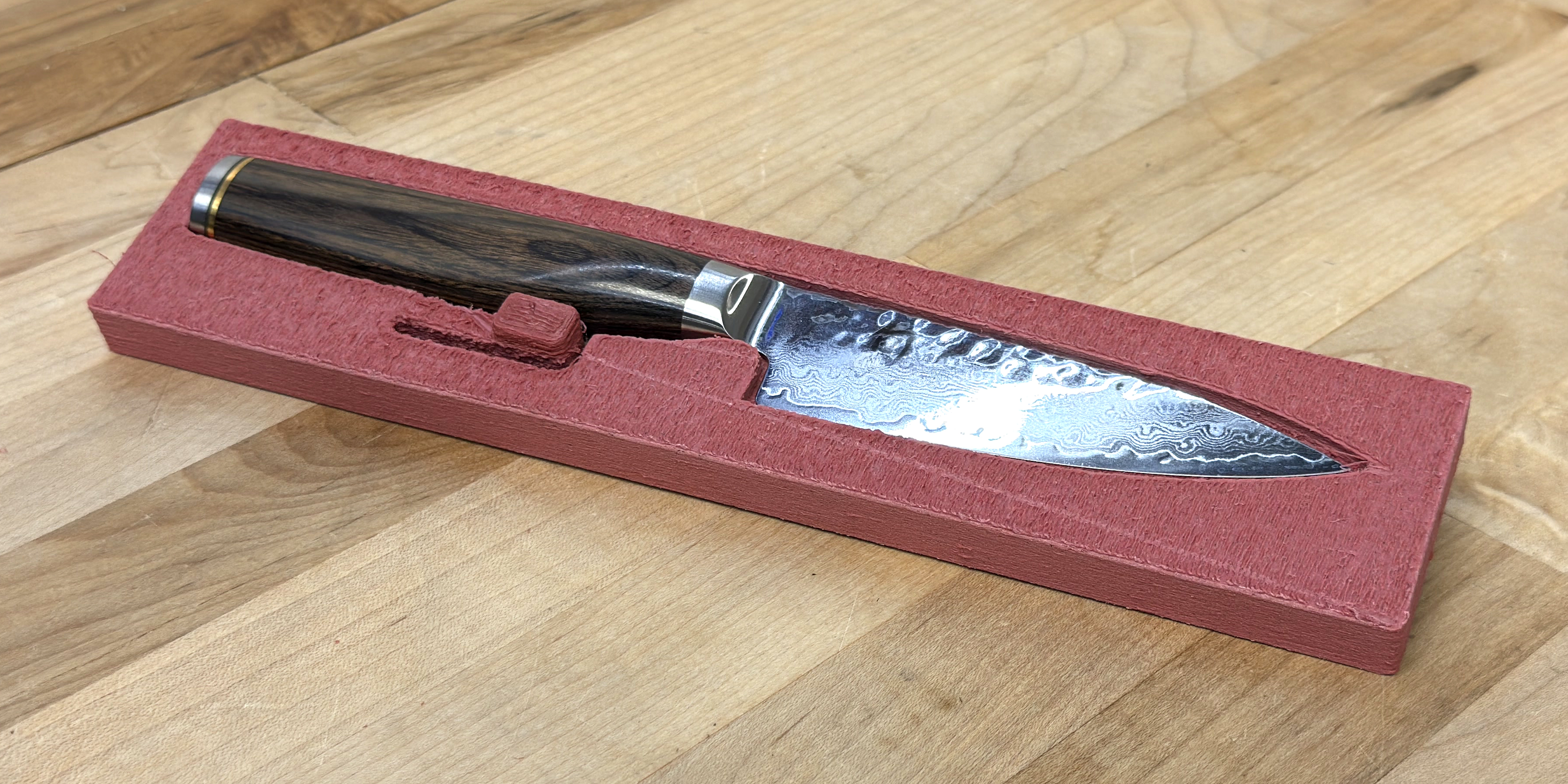
6.10.1.7 TimberFill, 0.4mm High Flow Nozzle
![]()
![]()
![]()
![]()
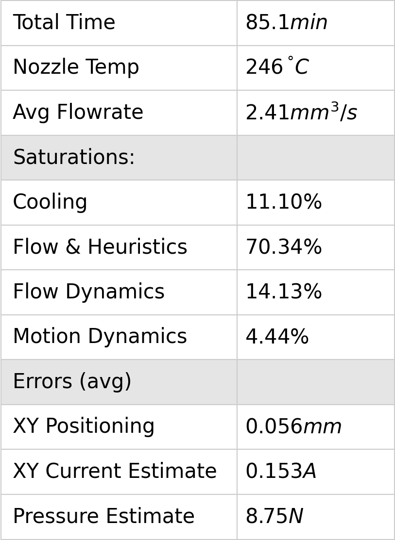
6.10.1.8 AluFill (67% 6061 Aluminum + Binder)
![]()
![]()
![]()
![]()

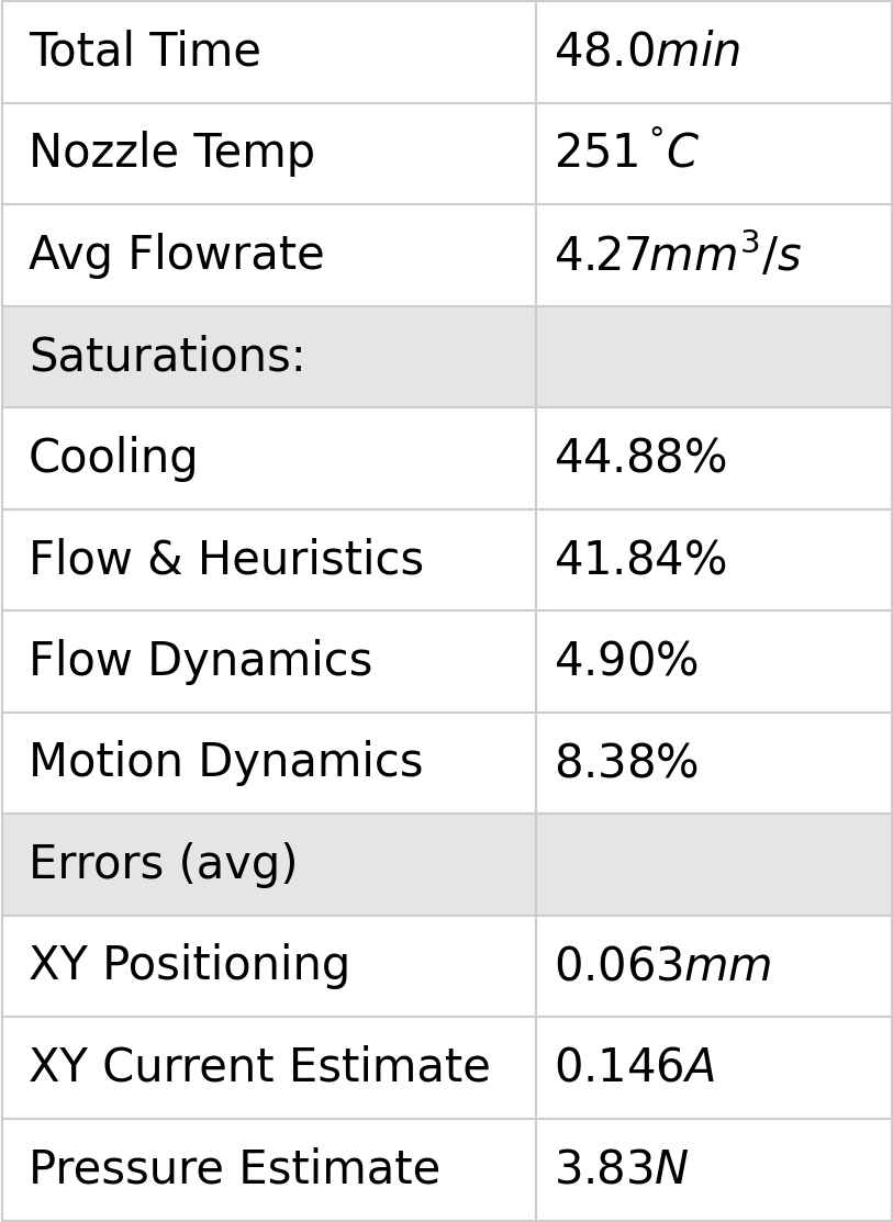
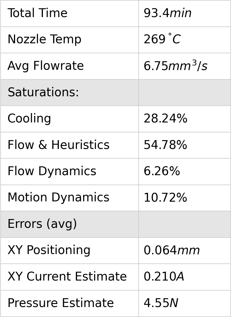
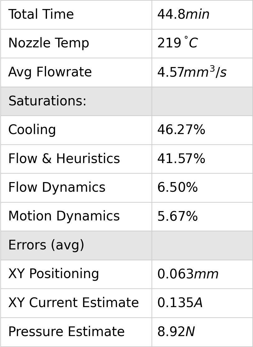
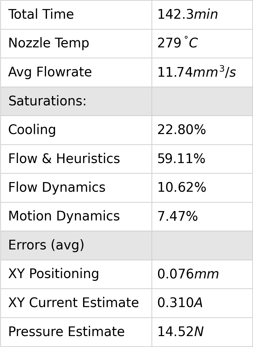
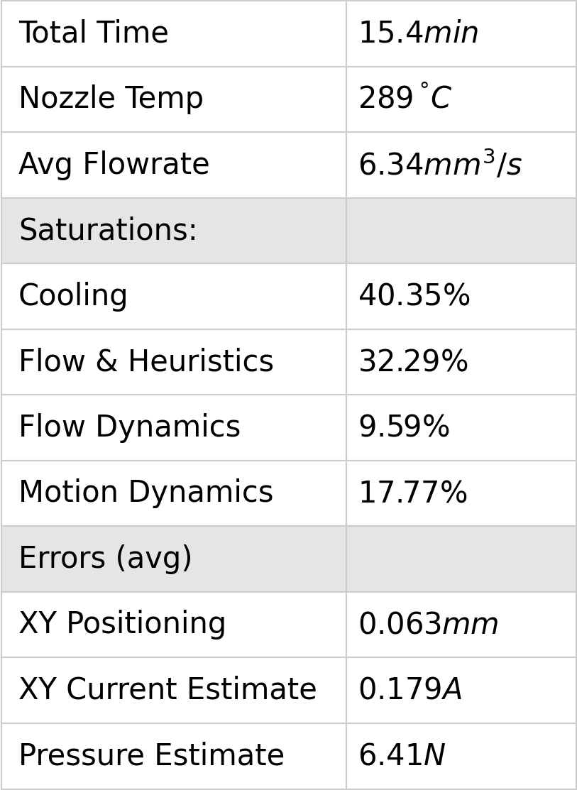
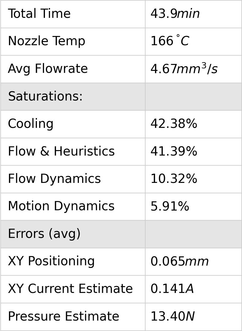
6.10.2 Model-Fit Quality
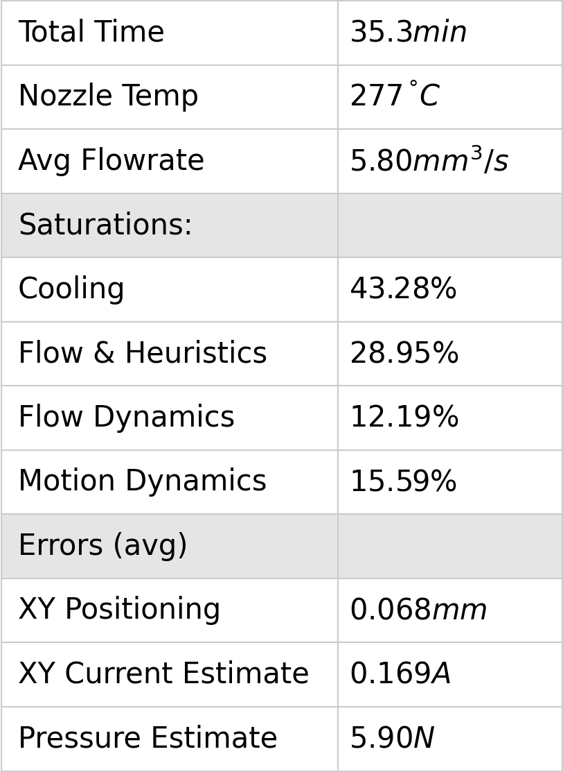
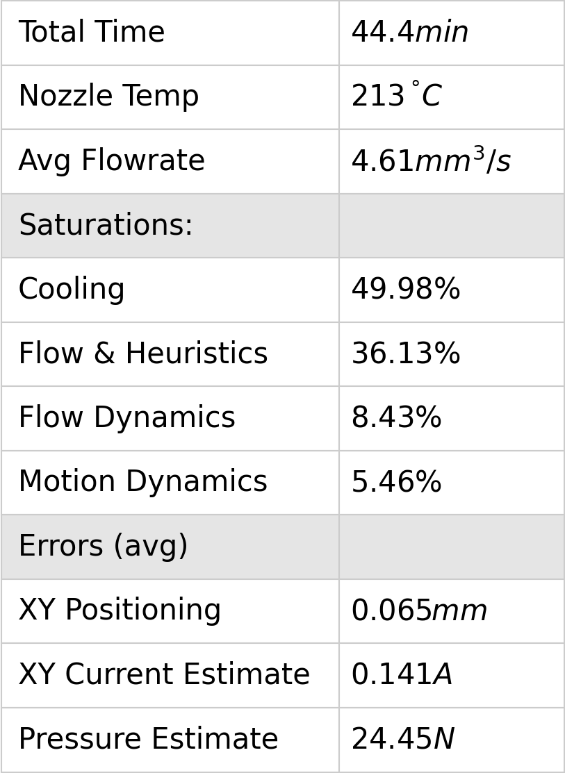
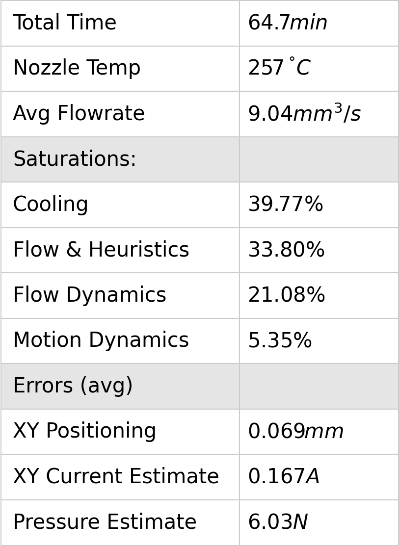
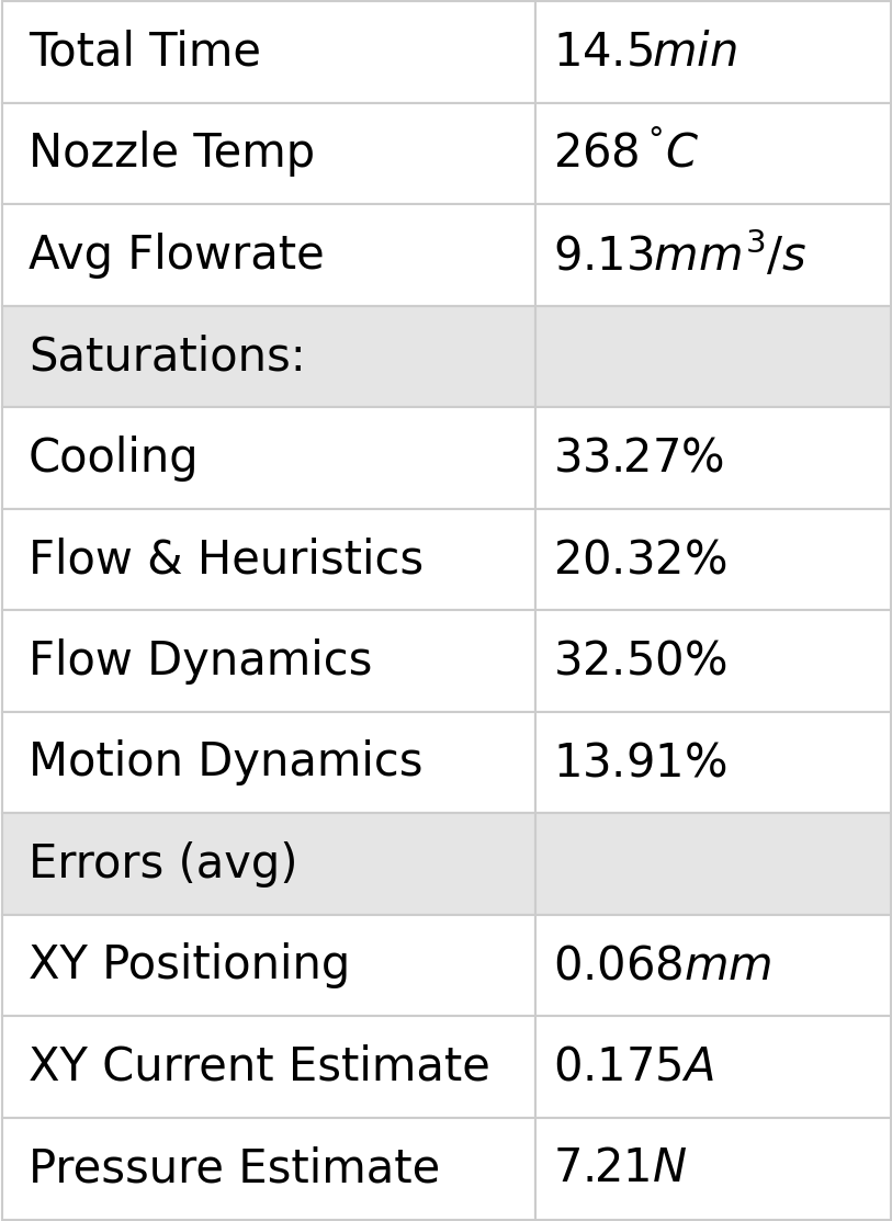
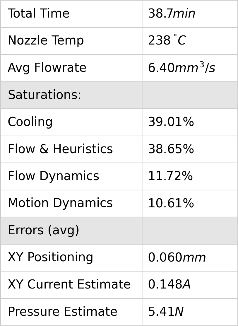
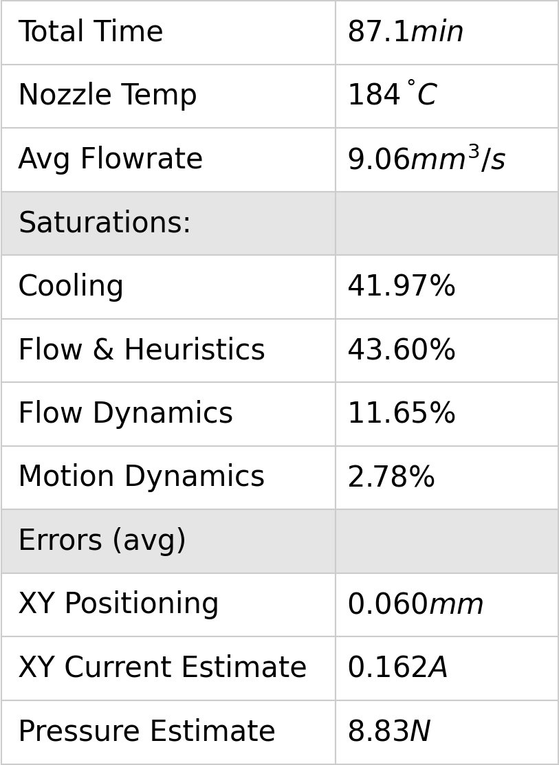
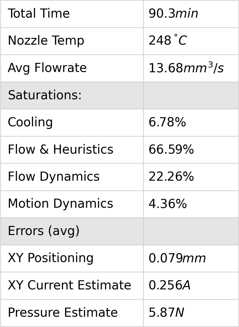
In each print above, I rendered a small table that includes average errors for XY Current and Pressure Estimate. These are end-to-end evaluations of our modelling workflow, and they are made using time-series data collected from the printer’s hardware and from the solver simultaneously. I look more closely at the XY Current error evaluations in 5.7.2 and I discuss the quality of flow model fits in Section 6.11.4.
6.10.3 Print Speed vs. SOTA
The workflow developed here increases speed over the state-of-the-art workflow, on average by \(141 \%\).
| Mat. | Noz. | Geometry | Total Volume | Our Time | SOTA Time | Speedup |
|---|---|---|---|---|---|---|
| \(mm^3\) | \(min.\) | \(min.\) | \(\%\) | |||
| PLA | 0.6 | 3DBenchy | 12773 | 48.0 | 53.0 | 110.4 |
| PLA | 0.6 | 3DBenchy 1.50x | 39737 | 93.4 | 104.0 | 113.5 |
| PETG | 0.6 | 3DBenchy | 12773 | 35.3 | 58.0 | 164.3 |
| PETG | 0.6 | Roadballs | 34687 | 49.3 | 68.0 | 137.9 |
| PCBlend CF | 0.6 HF | 3DBenchy | 13125 | 38.3 | 67.0 | 175.0 |
| PCBlend CF | 0.6 HF | Drone Fuselage Cap | 6119 | 15.4 | 23.0 | 149.4 |
| PCBlend CF | 0.6 HF | Drone Arms | 32247 | 60.4 | 80.0 | 132.5 |
| PCBlend CF | 0.6 HF | Drone Fuselage Halves | 42233 | 65.1 | 92.0 | 141.3 |
6.10.4 Qualitative Print Quality vs. SOTA
I did not develop a workflow to rigorously evaluate print quality against the state-of-the-art, but photographs below (our prints on the left, SOTA on the right) provide a simple basis for qualitative assessment.
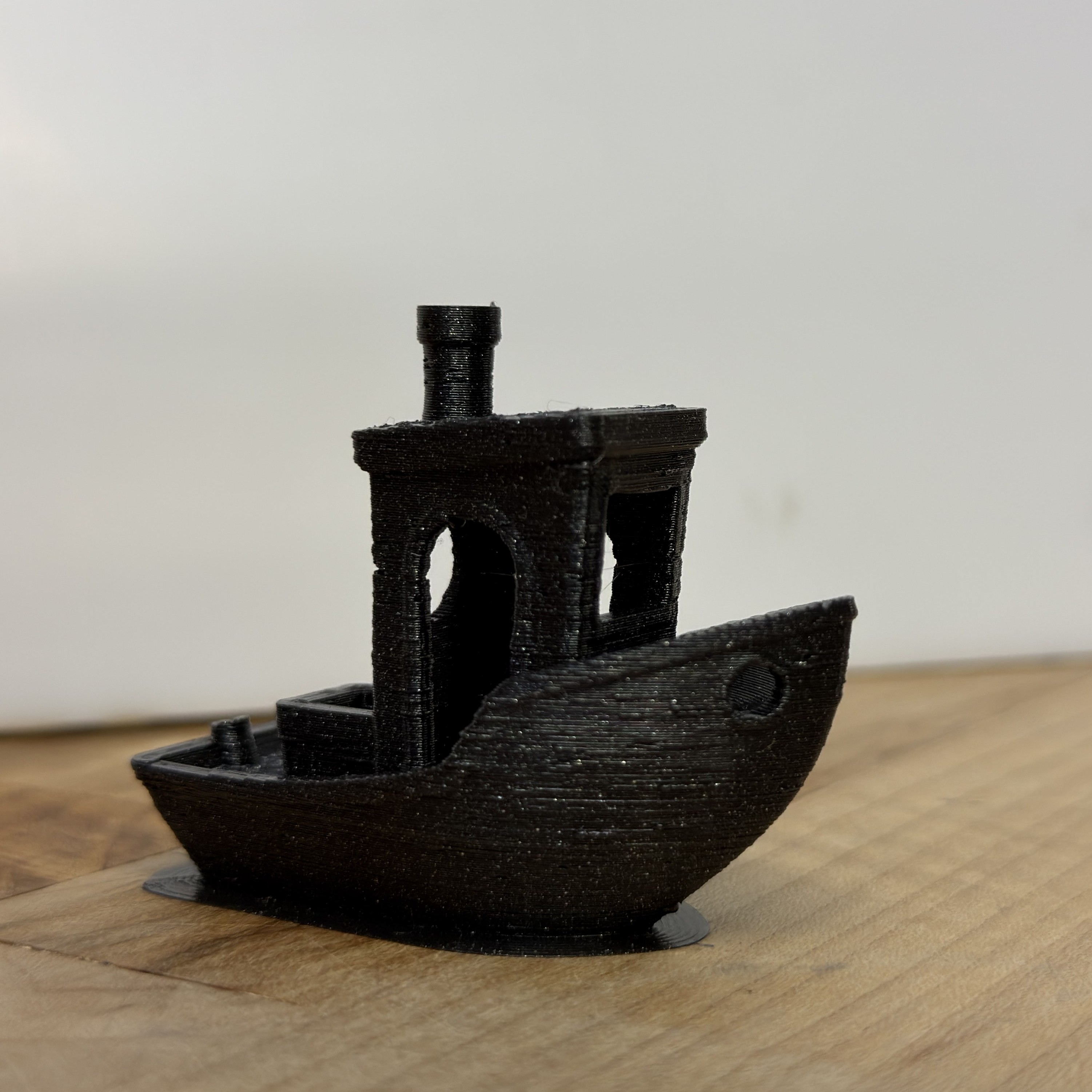
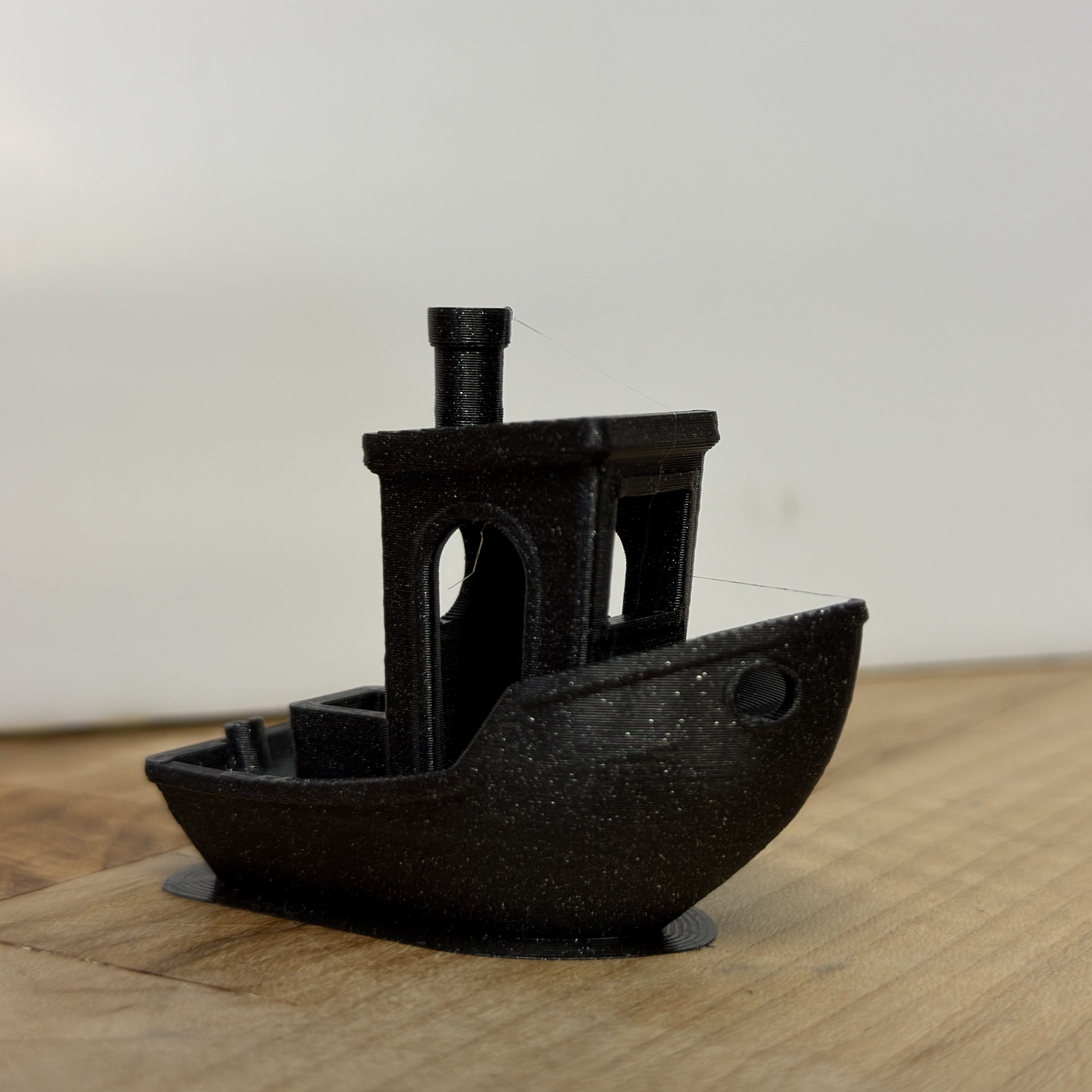
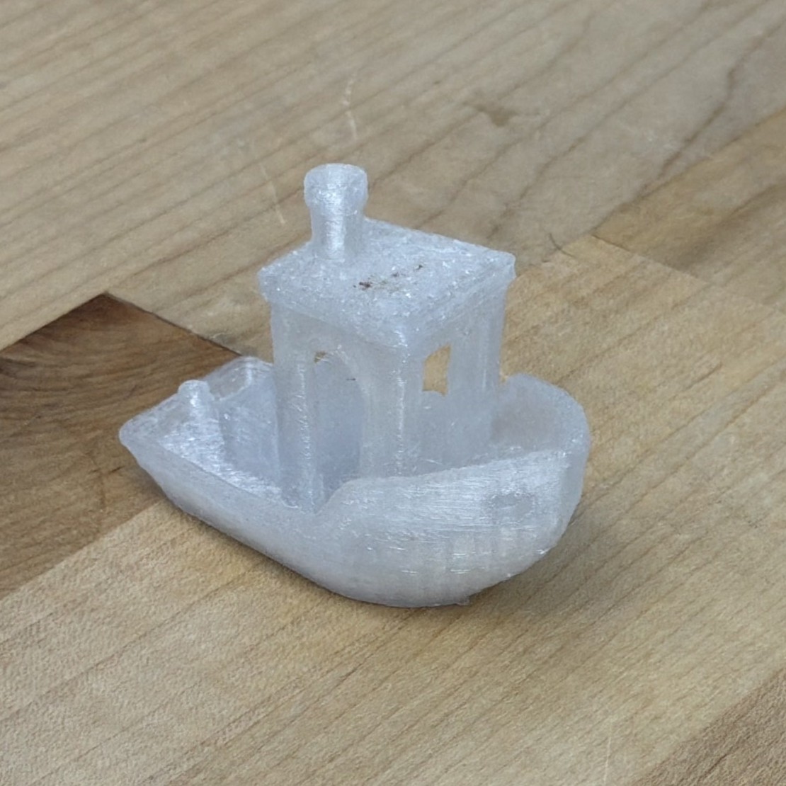
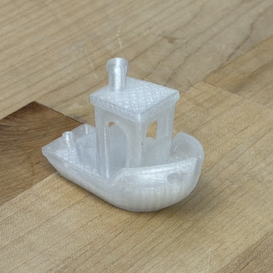
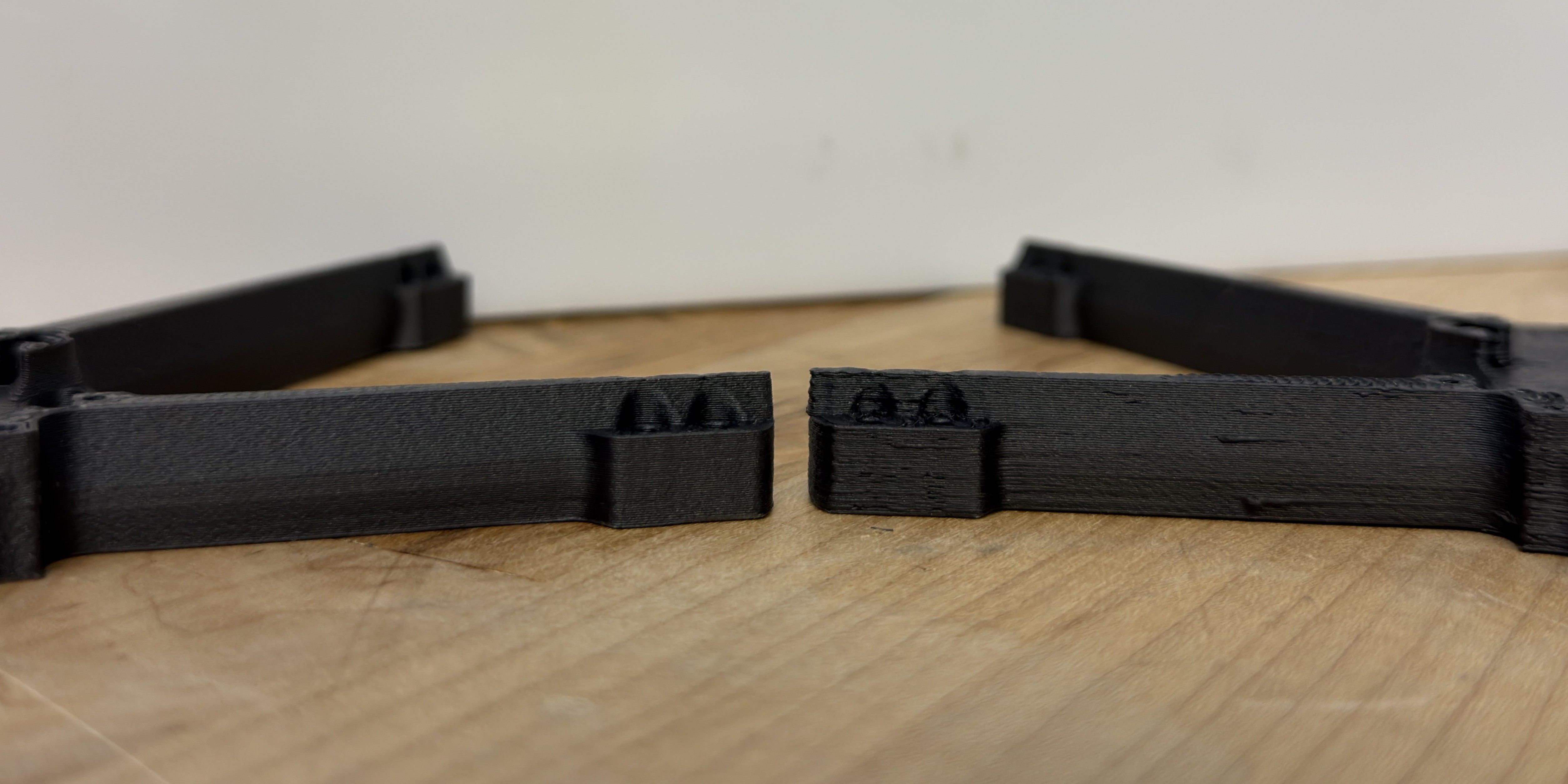
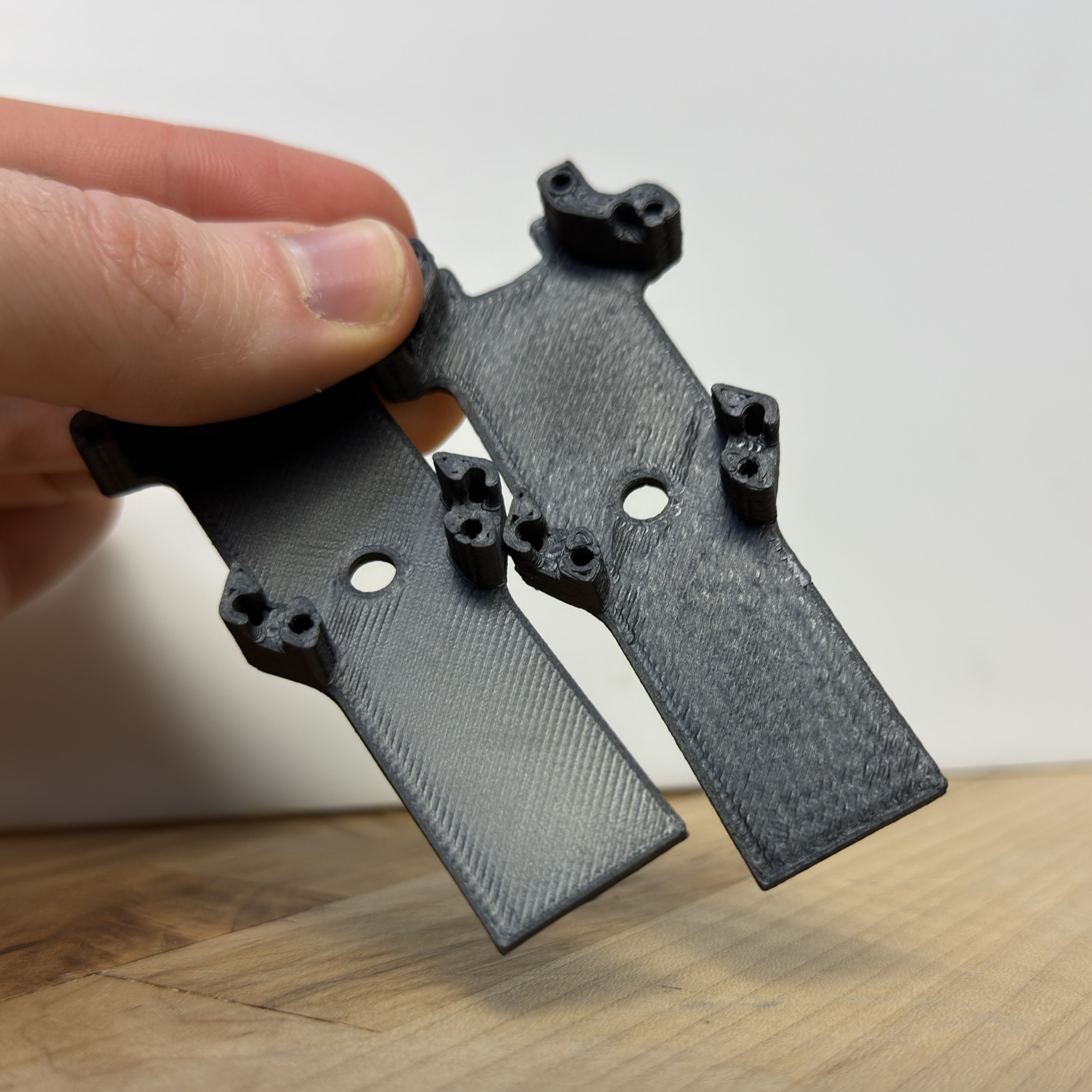
Overall, prints using our controller have many more artefacts than the state of the art.
6.10.5 Tables of FFF Results
6.10.5.1 Complete Table of Flow Models
- A Flow Model’s Minimum Temperature \(T_{min}\) is the temperature at which Maximum Flowrate is \(15mm^3/s\)
- A Flow Model’s Maximum Flowrate \((Q_{max})\) is taken at \(290^\circ C\)
- The springrate \(k_{sq}\) is…
| Mat. | Noz. | \(T_{min} \ (^\circ C)\) | \(Q_{max} \ (mm^3/s)\) | \(k_{sq} \ (220 ^\circ C)\) | \(k_{sq} \ (290^\circ C)\) |
|---|---|---|---|---|---|
| PETG CF | 0.4 HF | 197.7 | 73.1 | 56.91 | 21.33 |
| ASA GF | 0.4 HF | 188.9 | 71.1 | 34.24 | 7.67 |
| Timberfill | 0.4 HF | 151.2 | 80.3 | 16.21 | 3.24 |
| PLA | 0.6 | 181.1 | 54.0 | 25.83 | 9.19 |
| PETG | 0.6 | 193.4 | 53.9 | 24.20 | 10.91 |
| PLA | 0.6 HF | 175.0 | 69.3 | 26.66 | 7.89 |
| PETG | 0.6 HF | 200.5 | 57.7 | 32.82 | 12.41 |
| ASA | 0.6 HF | 193.8 | 58.4 | 28.19 | 7.32 |
| PETG CF | 0.6 HF | 188.0 | 77.5 | 42.44 | 16.92 |
| PCBlend CF | 0.6 HF | 235.4 | 53.5 | 53.61 | 20.83 |
| Nylon GF | 0.6 HF | 201.5 | 49.7 | 17.90 | 4.59 |
| AluFill | 0.6 HF | 209.9 | 146.4 | 19.88 | 13.33 |
6.10.5.2 Complete Table of Prints
| Mat. | Noz. | Geometry | System | \(T_{noz}\) | \(Q_{avg}\) | \(t\) | \(s_{cool}\) | \(s_{flow}\) | \(s_{extr}\) | \(s_{motn}\) |
|---|---|---|---|---|---|---|---|---|---|---|
| \(^\circ C\) | \(mm^3/s\) | \(min.\) | \(\%\) | \(\%\) | \(\%\) | \(\%\) | ||||
| PLA | 0.6 | 3DBenchy | Ours | 251 | 4.27 | 48.0 | 44.9 | 41.8 | 4.9 | 8.4 |
| SOTA | 230 | 4.02 | 53.0 | |||||||
| PLA | 0.6 | 3DBenchy 1.50x | Ours | 269 | 6.75 | 93.4 | 28.2 | 54.8 | 6.3 | 10.7 |
| SOTA | 230 | 6.37 | 104.0 | |||||||
| PETG | 0.6 | 3DBenchy | Ours | 277 | 5.80 | 35.3 | 43.3 | 29.0 | 12.2 | 15.6 |
| SOTA | 250 | 3.67 | 58.0 | |||||||
| PETG | 0.6 | Roadballs | Ours | 289 | 11.03 | 49.3 | 5.9 | 50.0 | 20.0 | 24.1 |
| SOTA | 250 | 8.50 | 68.0 | |||||||
| PETG CF | 0.4 HF | 3DBenchy^1 | Ours | 213 | 4.61 | 44.4 | 50.0 | 36.1 | 8.4 | 5.5 |
| PETG CF | 0.4 HF | Kleat^1 | Ours | 279 | 10.82 | 25.4 | 11.7 | 36.8 | 45.6 | 5.8 |
| PETG CF | 0.4 HF | Circuit Mount^1 | Ours | 257 | 9.04 | 64.7 | 39.8 | 33.8 | 21.8 | 5.6 |
| ASA GF | 0.4 HF | 3DBenchy^1 | Ours | 219 | 4.57 | 44.8 | 46.3 | 41.6 | 6.5 | 5.7 |
| ASA GF | 0.4 HF | Brake Duct^2 | Ours | 279 | 11.74 | 142.3 | 22.8 | 59.1 | 10.6 | 7.5 |
| Nylon GF | 0.6 HF | 3DBenchy | Ours | 230 | 5.03 | 40.8 | 47.6 | 27.0 | 18.1 | 7.3 |
| Nylon GF | 0.6 HF | Hood Latch | Ours | 268 | 9.13 | 14.5 | 33.3 | 20.3 | 32.5 | 13.9 |
| Nylon GF | 0.6 HF | Motor Mount | Ours | 238 | 6.40 | 38.7 | 39.0 | 38.7 | 11.7 | 10.6 |
| PCBlend CF | 0.6 HF | 3DBenchy | Ours | 289 | 5.36 | 38.3 | 49.4 | 33.4 | 5.8 | 11.5 |
| SOTA | 280 | 3.26 | 67.0 | |||||||
| PCBlend CF | 0.6 HF | Drone Fuselage Cap | Ours | 289 | 6.34 | 15.4 | 40.4 | 32.3 | 9.6 | 17.8 |
| SOTA | 280 | 4.43 | 23.0 | |||||||
| PCBlend CF | 0.6 HF | Drone Arms | Ours | 289 | 9.25 | 60.4 | 3.11 | 45.5 | 19.8 | 31.6 |
| SOTA | 280 | 6.72 | 80.0 | |||||||
| PCBlend CF | 0.6 HF | Drone Fuselage Halves | Ours | 289 | 10.24 | 65.1 | 2.9 | 54.5 | 12.6 | 30.0 |
| SOTA | 280 | 7.65 | 92.0 | |||||||
| Timberfill | 0.4 HF | 3DBenchy^1 | Ours | 166 | 4.67 | 43.9 | 42.4 | 41.4 | 10.3 | 5.9 |
| Timberfill | 0.4 HF | Moai^1 | Ours | 184 | 9.06 | 87.1 | 42.0 | 43.6 | 11.7 | 2.8 |
| Timberfill | 0.4 HF | Knife Holder^1 | Ours | 248 | 13.68 | 90.3 | 6.8 | 66.5 | 22.3 | 4.4 |
| AluFill^3 | 0.6 HF | 3DBenchy | Ours | 246 | 2.41 | 85.1 | 11.1 | 70.3 | 14.1 | 4.4 |
| AluFill | 0.6 HF | Circuit Heatsink | Ours | 238 | 2.29 | 59.4 | 2.9 | 77.9 | 16.5 | 2.7 |
| AluFill | 0.6 HF | Circuit Heatsink 1.18x | Ours | 246 | 2.88 | 83.8 | 2.2 | 76.7 | 18.2 | 2.9 |
6.11 FFF Discussion
6.11.1 Reducing Parameter Spaces
In the introduction of this section, I rendered a table of printing parameters taken from a state of the art slicer, Table 6.1. That contains 47 parameters, of which:
- 16 are either geometric or easily calculated based on nozzle width,
- 12 are translational velocities
- 7 are accelerations
- 3 are temperatures (nozzle, bed, chamber)
- 1 is directly filament flow related (maximum flowrate)
- 4 are retract related
Our workflow does not modify the geometry generation step of the state of the art, and does not set bed or chamber temperatures, so we are left with 29 free parameters.
Our workflow still relies on some human-in-the-loop tuning, and I lay out a similar table of these parameters in Table 6.5. It contains 21 heuristics or “manually” estimated values:
- 4 related to cooling
- 1 first layer rate
- 1 minimum flowrate
- 3 pressure scalars
- 8 motion scalars (current, and current slew rates)
- 4 extruder heuristics
In all, we have a similar total count of parameters. However, parameters in the state of the art workflow should be modified by hand for every new material, nozzle or machine. Our workflow uses models to mediate between this subset of heuristics and actual control inputs to the machine. While I was printing the parts above in Section 6.10.1, I dialled these heuristics in once for the machine (using PLA, over the course of about one day) and then left them alone for each new material or nozzle. Those values are the third column of Table 6.5. To be explicit, that means that tuning each of the print systems in Section 6.10.1 (11 nozzle and material combinations in total) from scratch in the state of the art workflow would have involved tuning up to 319 individual parameters. In our workflow, we can tune 21 parameters on one material and nozzle, and use models to extend that work automatically across new materials and nozzles.
To discuss, I want to go back to the compiler analogy that I made with Figure 1.4. In this analogy, the SOTA workflow amounts to writing assembly codes: parameters we set are directly implemented by the machine (subject only acceleration control). Our workflow is something like a compiler, combining high level and physically meaningful heuristics with models and optimization to produce the actual, low-level instructions.
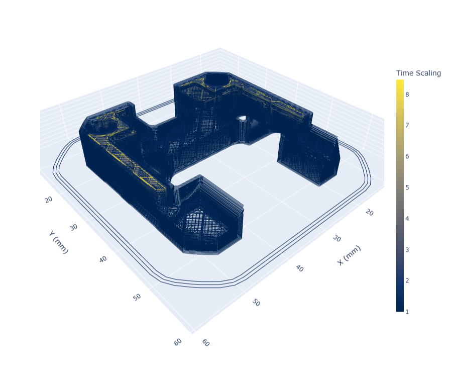
6.11.2 Learning from Printer Data Outputs
Whereas models on their own can tell us about how components of our system behave, the model based controller outputs can teach us about the system as a whole. During any print job, we collect numerous data streams from the machine and the solver that can all be used for analysis later - and with sufficiently accurate models, we can even do this with the system’s digital twin alone. Probably the most interesting way to process this data is to analyze (at every point in the part geometry) which aspect of the machine was limiting overall performance. This is shown below in Figure 6.55, where a few layers of a printed part are rendered with a colormap that corresponds to whichever system component was the most constraining on overall speed at that junction in the part. In Figure 6.56, the same data is rendered into bins showing how much time the printer spent during that job limited by each category.
The categories covered relate both to machine / motion models and flow models. Most dominant in this figure is cooling: tracks that have been slowed down to meet minimum layer time constraints. The second most dominant constraint are the flow models themselves, which are combined with some heuristics (recall Section 6.8). Then we have a series of machine related limits: inflow and inflow acceleration limits, as well as extruder current limits, are all related to the extruder motor’s performance and power budget. AB and Z motor current limits relate to our actuator’s performance, but also the machine’s motion system as a whole: reducing the occurance of these limits could involve increasing actuator size or decreasing friction or mass in the motion system.
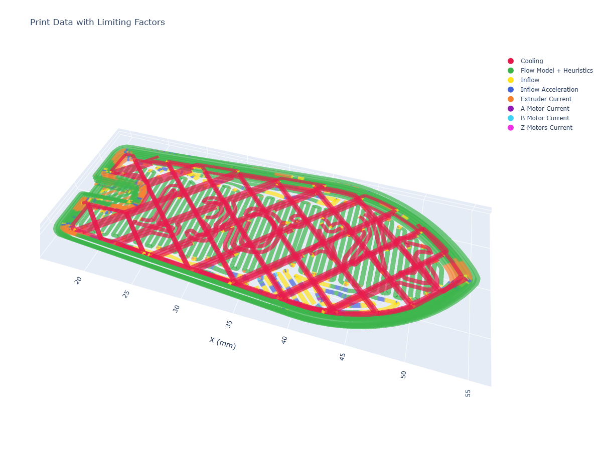
Machine design is a game of trade-offs: if we improve overall flowrates by i.e. increasing the extruder motor size, we add mass that the motion system must heft around through tight corners. If we decrease the size of the part cooling fan to reduce that weight, we remove cooling performance and need to add more time in each layer to counter it. Actually determining which of these trade-offs is the best to make is difficult to ascertain on pen and paper (or with a good spreadsheet) alone, since it is difficult to understand how often our various constraints are the main limiting factor, and it is difficult to understand how they couple with one another. These limits are also geometry dependent: if we print small, intricate parts we are more likely to be limited by the machine’s motion system and part cooling - whereas large parts are more likely limited by overall flowrates.
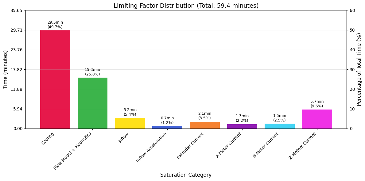
| \(s_{cool}\) | \(s_{flow}\) | \(s_{extr}\) | \(s_{motn}\) |
|---|---|---|---|
| \(28.0 \%\) | \(46.0 \%\) | \(15.4 \%\) | \(10.7 \%\) |
Using outputs like this, which emerge from the solver’s optimization loop (and our models), we can learn directly how all of these systems relate, and help us to make better machine design decisions in the future. I want to connect this briefly to what I mentioned in the introduction. In the state of the art, all of this learning is done on a purely intuitive basis. We have very many inputs (CAM parameters) and only a few easily measured outputs (total part time and quality). To learn how the inputs (and machine components) combine to improve or degrade either of those ouputs takes years of tuning on our own internal mental models. With model based control, we can read internal states and outcomes and learn directly where and how much each of our decisions is impacting outputs, basically tightening the loop on heuristic selections and machine design choices. I want to stress that I do not see this as a replacement for our mental models of machines and processes, rather as a tool to help more of us develop those models in more detail, with less time, and in a manner that could be more easily shared with others.
To generate these outputs, we compare time series data of each component’s outputs state with the relevant limit, for example motor current utilization vs. the maximum current available at that time. Each segment has a maximum velocity set via flow models and related heuristics, when that velocity is saturated we know that nothing else is constraining speed - and when that velocity has been scaled to meet a minimum layer cooling time, we know that the part cooling model has limited speed at that point.
Besides this more complex binning of output data to determine limiting components, we can also render individual traces to learn about our system. I have included a few of the most interesting traces in the figures below.
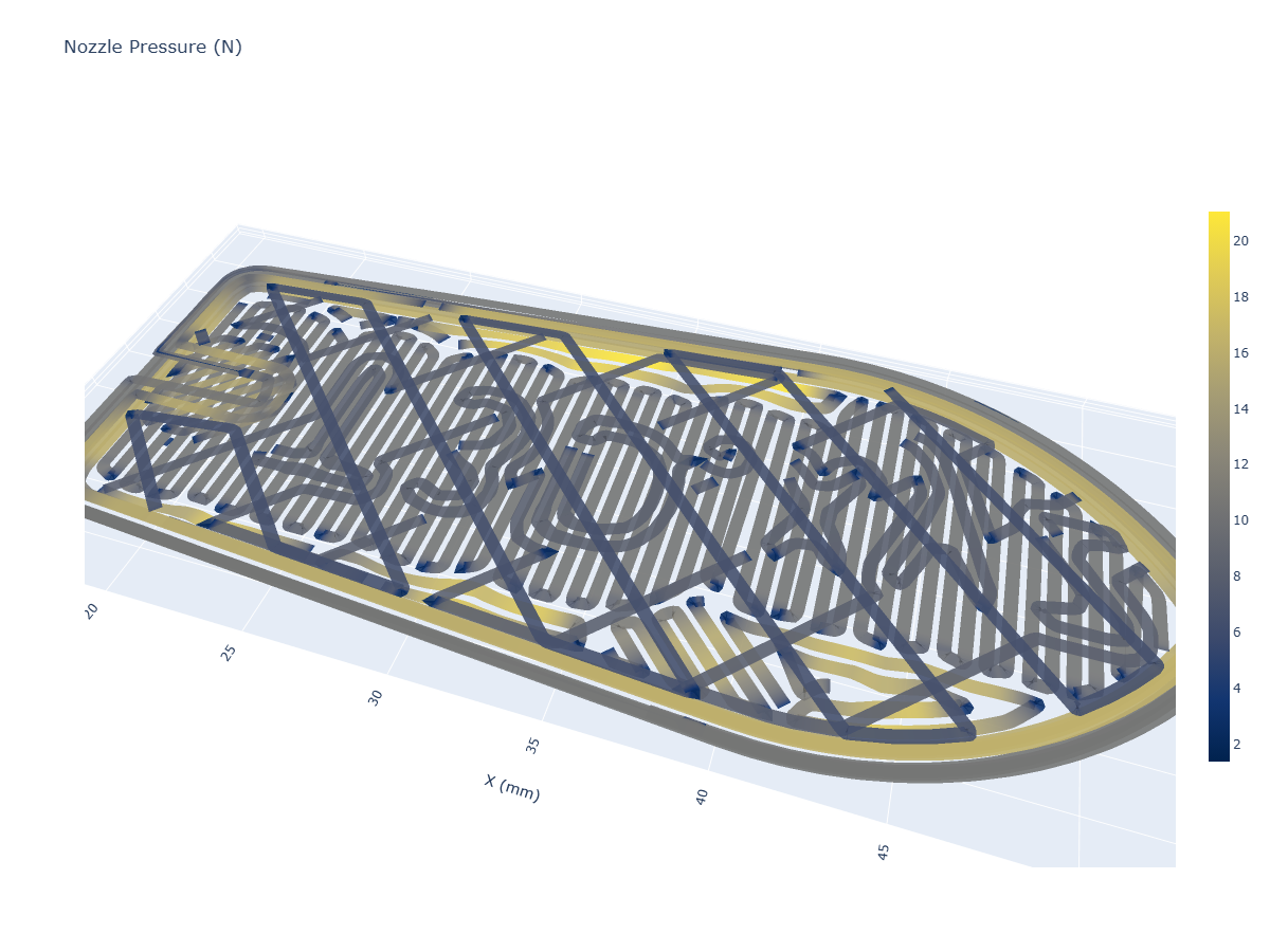
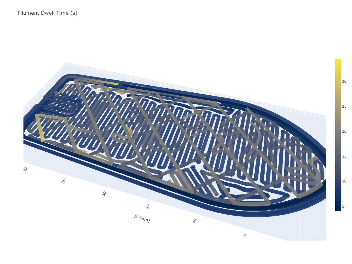
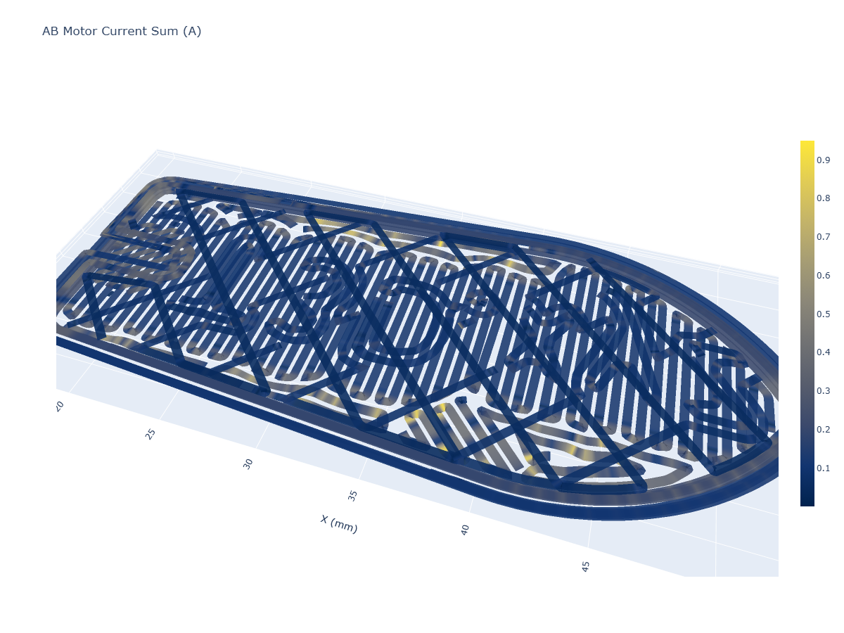
6.11.3 Learning from Flow Models
6.11.3.1 Comparing Materials
I want to make the simple point that models encode information about our materials that could be used to develop intuitive understandings of those materials. Below, I show three materials, each developed on the same nozzle and printer. …
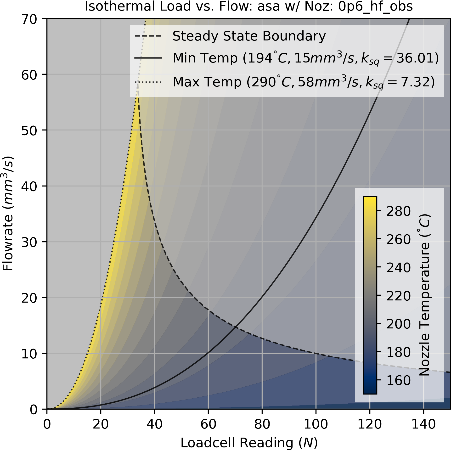
6.11.3.2 Comparing Nozzles
There have been recent advances in FFF nozzle design. The new state of the art nozzles include some internal geometry that improves heat flow into the filament. Models for flow can provide a basis for comparing these parts - below, I show flow models for PLA and PETG, using a traditional 0.6mm diamter nozzle on the left and a 0.6mm High Flow nozzle on the right. We can see that these nozzles do increase overall flowrates (as claimed) and also expand the size of the viable parameter space, moving the steady-state boundary curve away from the origin.
In Section 8.2, I discuss how figures or models like these could be used by i.e. nozzle manufacturers and customers to better articulate performance improvements or characteristics. For example a standard datasheet for a motor includes a torque curve, but in the state-of-the-art nozzle manufacturers only include scalar values for “maximum flow” for their nozzles - which are not even normalized across materials.
6.11.3.3 Comparing Fills
Before I started this project, I assumed that filaments with fiber fill (carbon or glass) were overall harder to print. Looking at their flow models, I was surprised to see that filled materials actually tend to have favourable flow properties. Models for PETG (without, and with) carbon fill are shown below, both with the same nozzle.
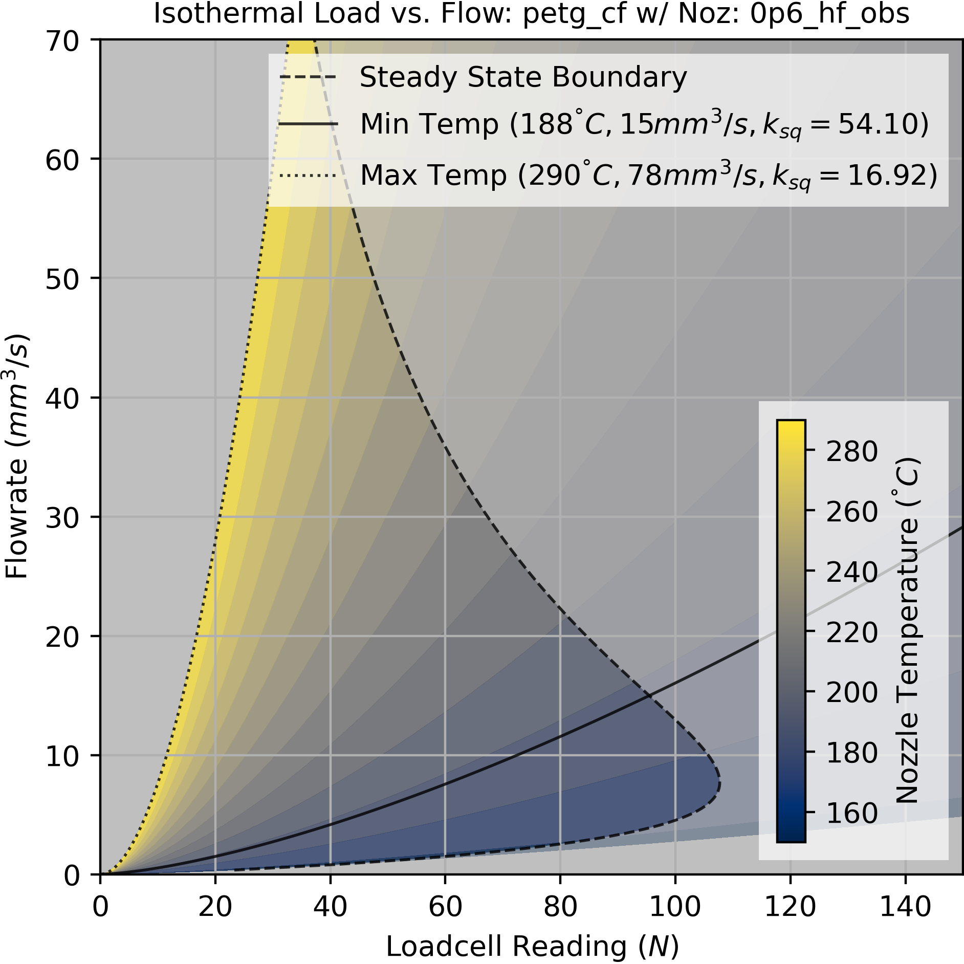
I think the phenomenology is that the fill, while increasing the viscosity of the material, also substantially increases its thermal conductivity. As noted, this leads to better flows overall because melt temperature is maintained at high flowrates. Above, we can see that the filled material moves the steady-state boundary away from the origin, and also substantially decreases the minimum flow temperature.
If you read the \(k_{sq}\) for each material, you will see that the fill has a higher springrate (\(16.9\) vs \(12.41 N/mm^3\)) at the same temperature (\(290 ^\circ C\)). We would expect this from the carbon fill, and it shows that maybe it is possible to extract some metric for material stiffness from our datasets.
6.11.4 FFF Model Fit Quality
Flow models are typically accurate only to 5-per-cent or so, and can be particularely bad over certain intervals in a part. I tally total model performance, per part, in the tables beside each print output (measuring average deviation of the pressure prediction from reality over the course of the print). Below, I show a time-series slice of data from the pressure system. We can see divergence in values for the extruder and pressure measurements, and even divergence in phenomenology.
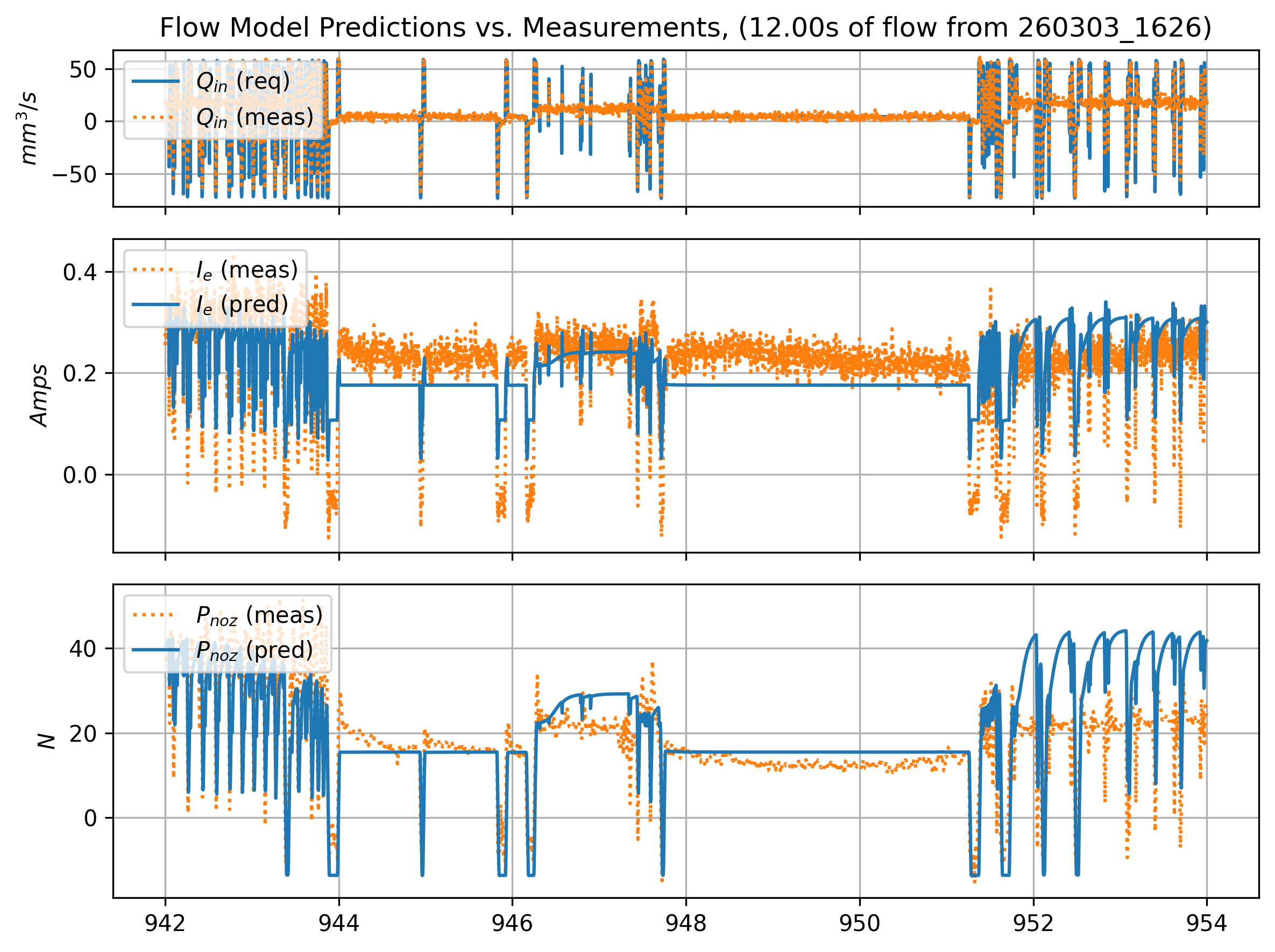
One result of this was that I had to implement the retract heuristic, which properly would be handled by the flow model properly driving pressure to zero. In Section 6.12, I cover a range of topics that might lead to improved modelling and operation of the hardware.
6.11.5 Resilience to Human Errors
A number of prints in Section 6.10.1 have a note: geometry was mistakenly generated for a 0.6mm nozzle. In these cases, I made the human error of labelling a flow model with the nozzle that I thought I had put into the machine (a 0.6mm High-Flow Obxidian nozzle), whereas I had actually installed a 0.4mm version of the same. The Obxidian nozzle is black, making it difficult to catch the nozzle diameter visually.
Some of these prints were hairier than usual, especially on top surfaces. I assumed that this was my own system’s modelling errors at play, until I realized the error that I had made. However, they all worked and on later inspection the model errors are not wildly out of the distribution when compared to the rest of the prints.
In these cases, the models used to process the files was still consistent with the nozzle that was used to print the parts: I swapped it before making models, not between model-making and printing. This means that the only thing amiss is that the print widths were configured for a 0.6mm nozzle, while the nozzle was actually 0.4mm. The system is resilient to this error since track widths are not dependent on nozzle diameter, only on total flowrate per unit of spatial displacement \((mm^3/mm),\) which can be forced out of a nozzle of any size.
It does mean that a key heuristic was missing, which is that track widths should not be printed that are substantially larger than the nozzle diameter. In Section 6.2 I briefly explained this: track widths are normally calculated over nozzle diameter, i.e. up to \(1.25 \cdot d_{noz}\) In these cases, track widths are about \(1.7 \cdot d_{noz}\)
As an experiment, I tried printing using the state of the art workflow, now intentionally making the error: I used a preset for each material in the two figures below, for a 0.6mm nozzle, but installed a 0.4mm nozzle in the machine.
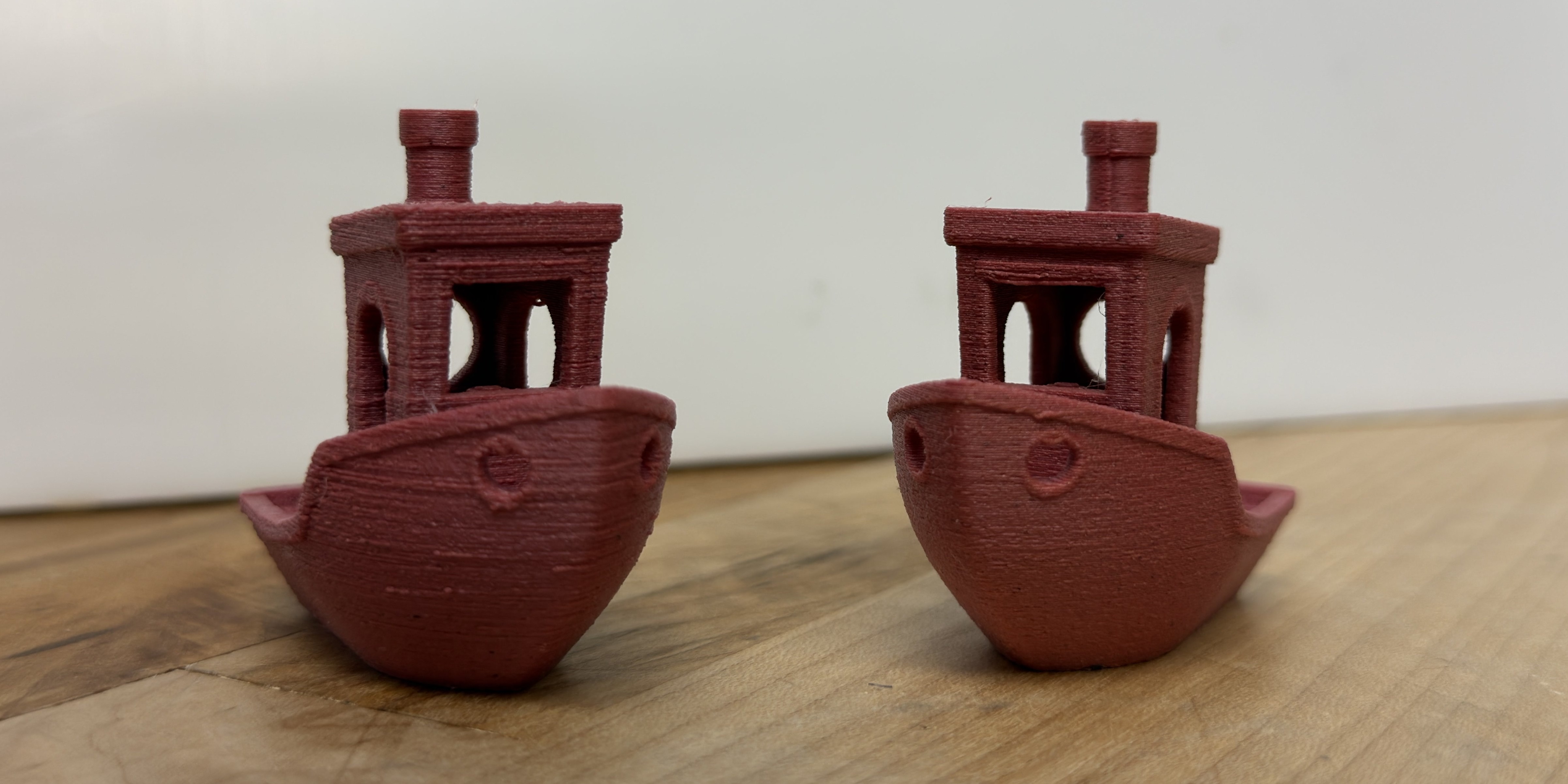
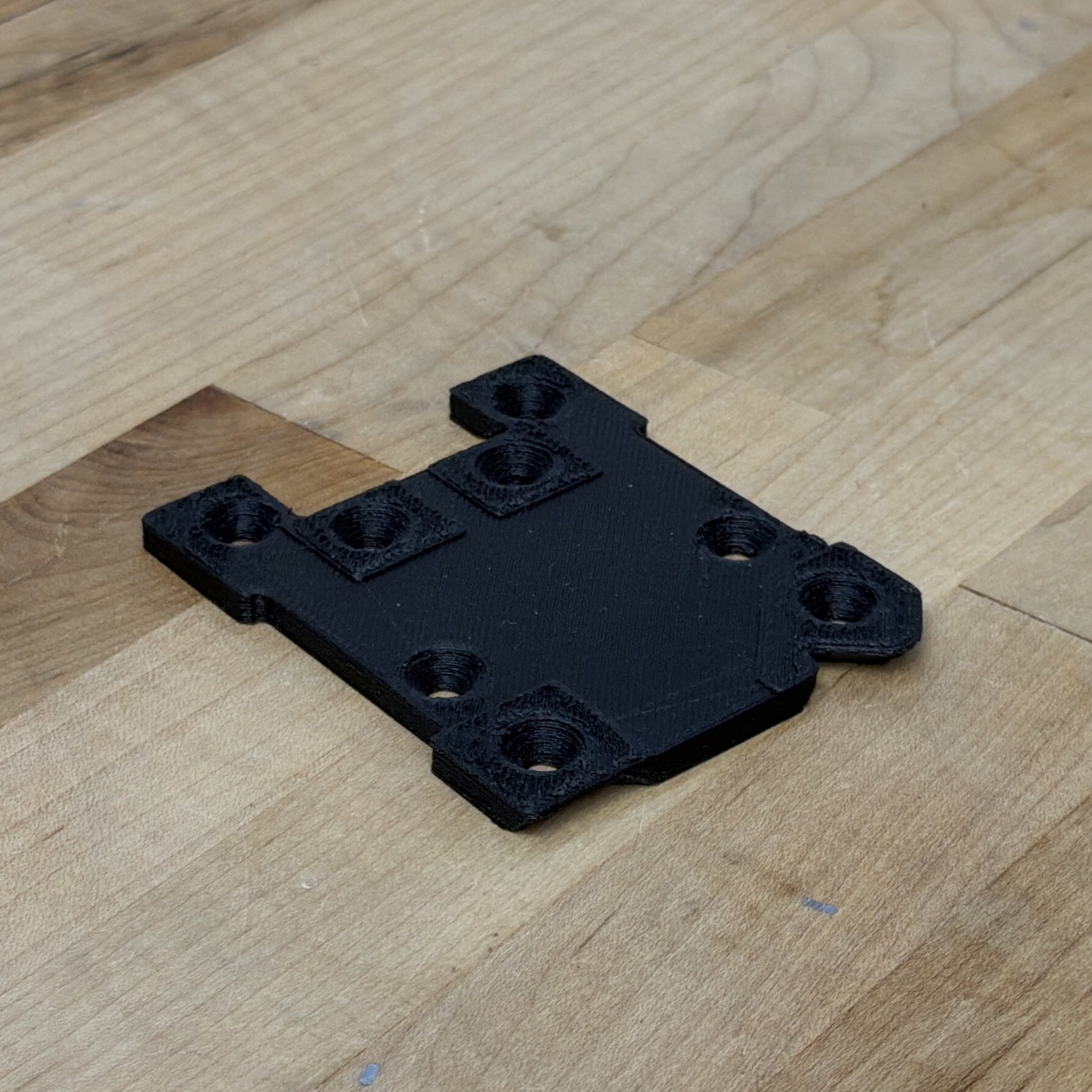
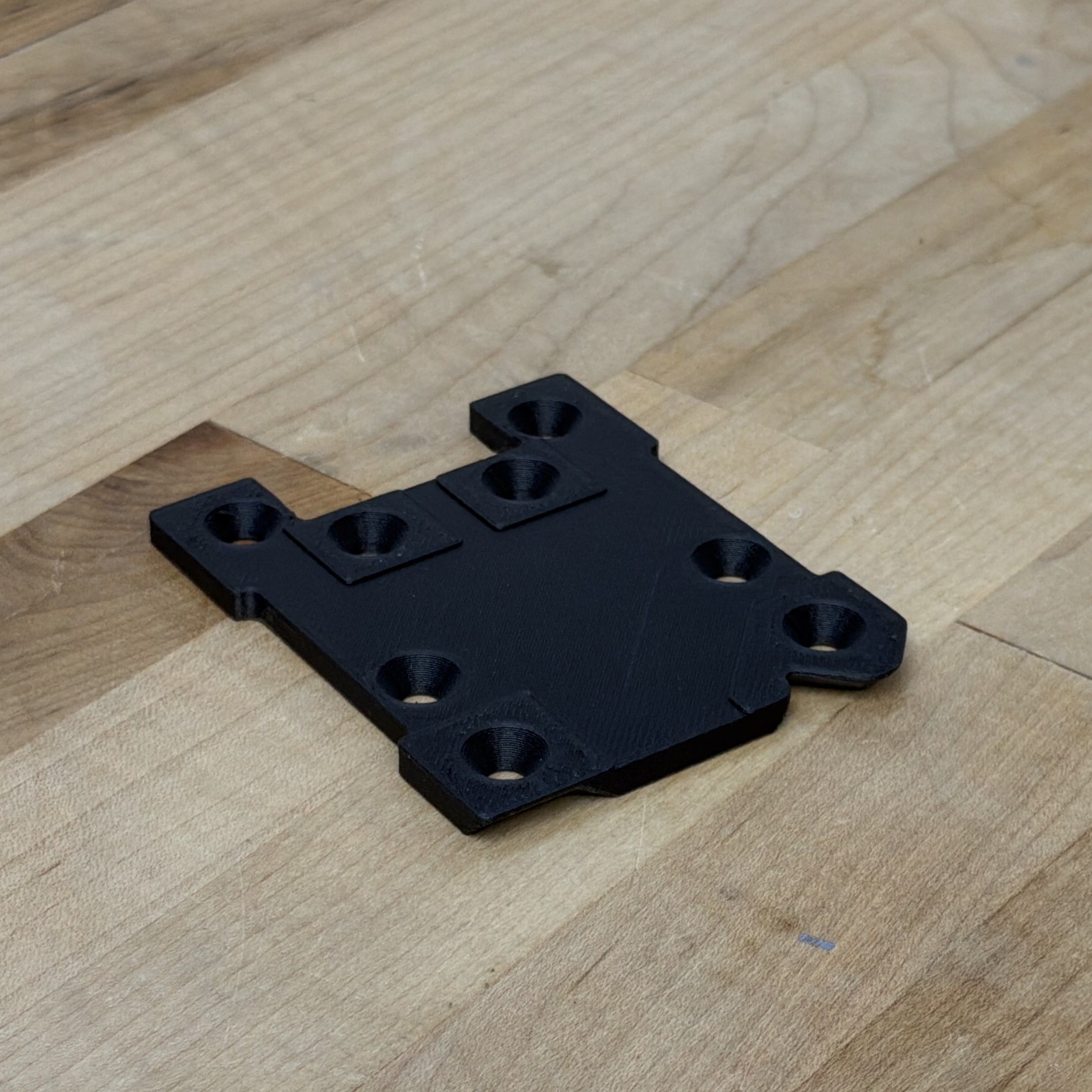
State-of-the-art prints were qualitatively still much better.
6.12 Future Work in FFF
6.12.1 Improved Modeling
6.12.1.1 Die Swell
Die swell occurs mostly when we extrude polymers when they’re not completely liquefied (which they never are?) or are extruded at extremely high pressures - i.e. one way to think about it is as the filament’s memory - when we extrude filament near maximum pressure (at low temperatures), it returns to about the same width as it was when it was solid filament - i.e. 1.75mm in our case.
This means that modelling die swell may reveal a second upper limit to flowrates, besides pressure generation and heating of the filament.
It should be possible to measure die swell, the microbolometer is perhaps the best place to start, but fitting widths using such small resolution is difficult. A proper vision system may be required.
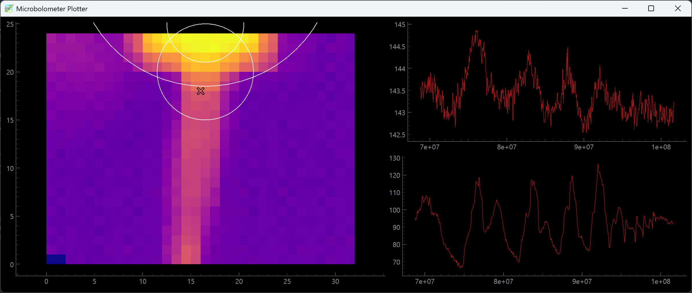
6.12.1.2 Cooling Model Fitting
If we see anything from our print data and i.e. Section 6.11.2 it’s that cooling is (very often) the most saturated limit. However, our cooling model is perhaps the least well developed out of our collection, missing estimates for filament conductivity, cooling to air, and missing entirely cooling beyond the immediate layer.
The microbolometer is potentially the best tool again for this research. Since its frames are time-synchronized to the motion system, we should be able to use them to recreate a 3D thermal history of the printed part. That, or simpler strategies (like measuring the average temperature of a part surface, during printing under variable fan parameters) could get us started improving our cooling model estimates.
6.12.2 Properly Combining Flow and Thermodynamic Models
In Section 6.5.5, I showed how I interpolate between steady-state and isothermal flow models. This step aids greatly in pressure prediction because FFF melt flows are, in practice, constantly changing temperature.
However, the modelling strategy (interpolating) doesn’t lend itself to “generic” machine data. Instead, it works only when we carefully develop a test routine that includes time-series data from either steady-state conditions or isothermal conditions.
After building the solver’s flow temperature calculation step in Section 6.9.2.1, I can now see that modelling the system directly as a thermodynamic system plus a temperature varying model for isothermal flow, which sounds oxymoronic but is actually exactly what we developed in Section 6.5.4 (the model relates pressure to flow instantaneously, so is isothermal in that sense - but it has different parameters across temperatures).
Modelling the thermodynamic system directly may have knock-on benefits. Its free parameters are values that we are interested in finding anyways: filament heat capacity is in there, as are some parameters we estimated for the cooling model (filament conductivity, heater block heat capacity, etc).
Here’s another upside for this task: nozzle thermal control is still done mostly with simple PIDs. Developing better controllers for the nozzle itself requires finding, again, those same parameters: heater block and nozzle heat capacities (and our existing power measurement) are critical also for feed-forward terms in thermal controllers. To date, these are not so important because we rely on the heat capacity in the heater block being much larger than that of the melt flow to simply smooth all of this out - then just about any PID gains will work well enough to keep the nozzle at the setpoint.
However, there is ongoing work in developing inductive nozzles for FFF. These have much less thermal mass, and so can change temperature much faster. I expect that these will become the new state of the art over the next few years. These especially will require better thermal control. They also present us with the opportunity of quickly changing flow temperature during a print.
Given the results here that cooling of prints is a major driver of overall print time, and that nozzle temperature has the largest overall effect on flow dynamics, the opportunity with fast thermal slew rates would be to optimize nozzle temperatures over the course of a print: larger layers with warmer temperatures, smaller layers with colder temperatures. If thermal slew-rates are fast enough, we could even imagine ramping nozzle temperature along with acceleration to produce prints with roughly equal extrusion pressure throughout.
6.12.3 Continuous Improvement and Deployment
One of the things that makes this system unique is that the measurement equipment and the process equipment are the same. In most materials modeling paradigms, we use offline hardware to characterize samples, develop process parameters for feed-forward controllers, and then deploy them. In this case, we use much lower fidelity instrumentation but can use it continuously to generate “an embarrassment” of data (Sutton 2019), about one gigabyte per hour.
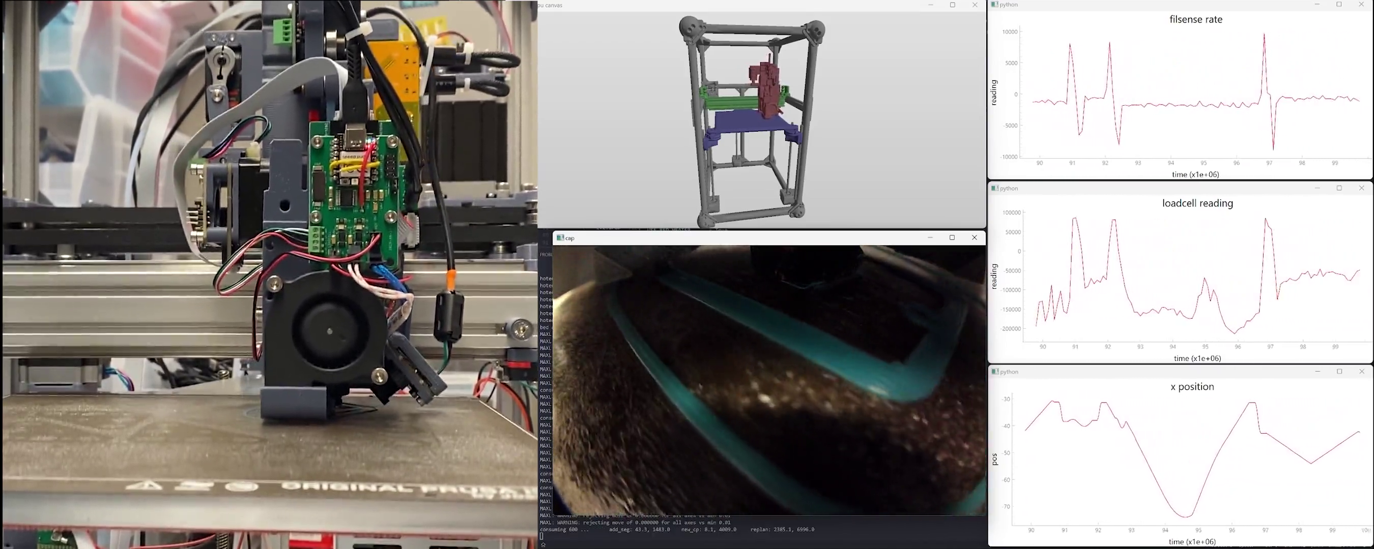
In Section 5.7.3, I showed that we can successfully re-fit motion models from data generated during machine operation. This is particularely valuable for machines whose damping and inertial terms may change over time, as is often the case: grease dries out, belts are tightened or loosen, and (i.e. in a milling machine) masses can change even over short time spans. We should be able to do the same for our process models, continually refining flow, cooling, and extruder models as we amass more data.
However, there are a number of challenges in this regard that prevented me from implementing it.
- Where we use a steady-state and isothermal flow model (and then interpolate between them) (having carefully designed tests to contain data in each of these regimes), data taken during prints is almost always between these two states. That makes Section 6.12.2 a prerequisite for this step.
- Much of the data is redundant: we would want to be able to continuously improve without eating harddrives. models are made exactly for this (compression), but when we re-fit we want to keep some older samples to avoid over-fitting only on new data… could compress over state spaces (collect samples in states i.e. speed where data is sparse): total set of states in the machine is pretty high dimensional, and some time dependence (!)
6.12.4 Pareto Frontier Printing
The key tuning knob in the optimum nozzle temperature step is picking our target layer temperature \(T_{targ}\) - if we favor “hot and fast” prints that may be somewhat slumped (but stronger), we can dial this up: the minimum-time optimization will be penalized less for warmer flows (as minimum layer times will be shorter). If we want precision above all, we can turn this down and we will see the opposite result. This makes up one axis in a theoretical pareto frontier, which trades strength (at the cost of precision) for speed.
While I do not develop this, could formulate trade-offs for precision, speed and layer strength by defining optimal results for each. Optimal speed is obvious: we measure total time. Overall precision is a strong function of our cooling target (and overall flow speeds, slower flows being more predictable). Layer adhesion / part strength is a function of the layer interfaces’ thermal history, which I have shown can be modelled ~ basically just using layer times (we just need to integrate interface temperature over time). What is missing from the current work is a characterization of how much layer strength is gained from a given increase in interface temperature / time, and how much precision is gained from slowing down and over-cooling parts. However, I think that good heuristics could be developed in these cases, and the literature contains a slew of studies on each topic.
We could also develop this more completely to scan a print from bottom to top layers, analysing an ideal temperature for each layer such that print speed is maximized while the layer is sufficiently cool before the next begins. For example a print with large layers near the bottom and small near the top should begin with large nozzle temperatures and slowly cool as it approaches the small, detailed sections. This would require models not only for part cooling, but for the available thermal ramp rates of the nozzle. New printers are also being developed that use induction heating of the nozzle which greatly reduces thermal mass and enables much faster thermal response. These could be exploited to very quickly change nozzle temperature layer-to-layer or even feature-to-feature in a print. Lookahead solvers that account for short-term dynamics (acceleration, pressure) and longer-term dynamics (thermals) could presumably be developed to suit.
From here, I think the future of FFF printing is bright - I know that there are many others working in this domain, and (luckily for the public good) many of the bottlenecking patents have expired4. Despite the onslaught of new strategies being developed for additive (laser bed fusion, binder jetting, etc etc), FFF remains extremely useful, relatively easy, cheap, and (as we see here and elsewhere) capable of producing excellent parts whose performance is similar to injection moulded components (and using the same low-cost materials).
6.12.5 Improved Solving
- it’s easier to write dynamics down as time series / ODEs - unfortunately for this solver we have to manually transcribe from those representations into “backwards” looking models. bummer, and it seems like other MPC solvers don’t have the same constraint: so what’s up with that?
- solver is actually largely offline - it aint really MPC, but “properly” done it would be,
- alternately, simulations of entire prints should be possibe (fits easily on the GPU), to anneal over i.e. all time dependencies for thermodynamics, etc
- like, this thesis talks a lot about making headway in removing blocks from
References
FFF: Fused Filament Fabrication is the nomenclature preferred by academics for the 3D Printing process of extruding plastic filaments through a hot nozzle which typically goes by another three-letter acronym, that happens to be trademarked by a 3D Printing firm who shall not be named.↩︎
Side note: developing an intuition for the Watt is a valuable engineering practice… recall that a typical incandescent bulb is rated to 100W and about 95% of those Watts are coming out of the bulb as heat energy… probably don’t touch it directly, but sticking your hand close to the bulb will give you a sense for the amount of energy that “100W” is.↩︎
The subreddit in question is reddit.com/r/FirstLayerPorn.↩︎
For example Stratasys held a patent on enclosed build chambers and so for about 15 years most FFF companies couldn’t put their machine in a box (which greatly improves part warping, and makes the printer less susceptible to i.e. a drafty room). Some readers may be wondering why I keep calling it FFF - well, the other acronym is trademarked by the same company. This is all fair game in today’s patent law ecosystem, but a clear case where our old laws (developed in an era where technological advancement was more costly and took place in longer cycles) have become outdated. Not to mention a changing global order, especially in manufacturing, where some of the main participants are developing equipment within completely different legal frameworks - given the difference in the two worlds’ approaches to IP law it is no surprise to me that they are able to innovate at such an outstanding pace. Notes should be taken…↩︎