3 PIPES and MAXL: Programming Models for Modular Machine Control
3.1 Chapter Introduction
The first question that I posed in Section 1.3 was about developing the systems architecture that would enable feedback-based digital fabrication workflows. These workflows span high and low levels of compute, and across heterogeneous networks of embedded devices. Modularity across hardware and software makes it easier to develop machine systems that can be reconfigured in model-building and model-use workflows and lets us quickly add new instruments to our hardware, but it also requires that we develop a programming model that is consistent across those levels.
Our programming model needs to work for two basic tasks. The first is to configure machines, i.e. make sense of which devices are in the network and connect them to one another according to some control logic. This will include configuration of software modules throughout the system, but we will want to be able to do this without (for example) re-compiling and flashing firmwares, which is time consuming, cumbersome (especially on large and complex machines), and can easily lead to misalignments between firmware and software configurations. The second is to task that configuration, i.e. deliver trajectories to machines, home and jog them, etc - tell them what to do.
To accomplish these two tasks I wrote PIPES (for Piped Interconnect for Physical and Experimental Systems). PIPES runs on top of OSAP and is responsible for naming and describing software objects, building and modifying systems representations, configuring data flows between objects, and remotely calling software objects. PIPES uses a dataflow programming model to configure and represent real-time control, but also mixes in scripting tools that make the tasking problem easier. PIPES’ configuration tools are also presented as a software API, so that scripts which run machines can sequentially configure them programmatically, and then run those configurations.
Within that framework, we need to build motion control as a central application. The challenge in this regard is twofold: first, we need synchronized execution of a planned trajectory in our distributed modules. The basis for synchronization is OSAP’s clock sync service (Section 2.2.4.2), but we still need to write those trajectories and interpolate them. We also want to build controllers for a range of machines from a shared core of motion control components rather than re-writing them whenever we build a new machine. Finally, we need to develop motion control in a manner that allows us to uncover realtime states that are normally hidden beneath GCode, as I dicussed in 1.2.4.1. For these tasks I wrote MAXL (Modular Acceleration planning and eXecution Library); it develops motion controllers as dataflow graphs. We can then use PIPES configurations of MAXL blocks to combine kinematic transforms and corrections, lookahead planners (5.2.1 and 5.6), and a host of other motion planning utilities (3.3.3) into new controllers.
So, in this chapter: I will explain how PIPES (3.2) and MAXL (3.3) work (and how we write programs for them), and then how they enable us to collect time-series datasets 3.4.2, program and task machine systems (3.4.3), and flexibly deploy across a heterogeneity of kinematic systems (3.4.5) and in other mechatronic systems.
3.1.1 The Partitioning Problem
Unfortunately for everyone involved, it is impossible to make a perfect computer network. Any time we send a piece of data from one device to another, it takes some time to get there (delay), and requires some extra computing power to serialize, transmit, receive, route, and deserialize (overhead).
Network performance is also variable: if a link is congested its performance will decrease nonlinearly (i.e. slowly at first and then all at once) 1. Link performance is also dependent on “out of band” disturbances i.e. the electromagnetic environment. I was once debugging a packet loss issue for nearly half of a day before I realized that the cable (containing UART over RS485) was lying on top of a switching power supply, which was emitting noise in around the same frequency of the link’s bitrate. I moved the cable and the performance was restored. Wireless links are the same: too many cellphones in a room and your bluetooth headphones might stop working2.
All this to say that no matter how much engineering we do in our network layers, they will always be less performant and more importantly less deterministic than digital control (i.e. where all control elements are in the same CPU), because moving data into and out of a computer’s own memory is always faster than sending it over a network. This adds timing overhead to our controllers that are not present in digital controllers, which in turn reduce the bandwidth of our control algorithms (2019) (2012) (2002). Some of these challenges can be overcome by distributing models throughout a system, trading computation for bandwidth (Yook, Tilbury, and Soparkar 2002), and there are of course many cases where the advantage of being able to add more total computing to a system via networking is beneficial3.
In this chapter, we are contending with what I have been calling the partitioning problem - given some distributed system (a machine, say), how do we split the requisite tasks amongst some set of devices (motors, sensors, and a coordinating computer(s), for example), such that we have acceptable and scalable performance. I take for granted that flexibility is of primary concern: we want also to be able to make many different systems by adding and removing components from the network. We have other real constraints: we cannot run motor controllers or sensors on our laptop because it does not have the requisite low-level interfaces (or timing guarantees). Nor can we run high level languages or algorithms deterministically on embedded devices: they do not have enough compute power, or access to hardware accelerators like GPUs. The lines between these two halves are blurring in recent years, with multicore microcontrollers emerging and small, headless single-board computers (sometimes with AI accelerators) becoming available. Microcontrollers are also becoming ever more powerful, meaning that we can simultaneously do more computing at lower levels and return more data to higher levels.
In this framing, PIPES (3.2) presents tools for looking at partitioned systems, making sense of their global structure even if parts are in variable locations and then MAXL (3.3) builds motion control in a manner such that the controller can be flexibly partitioned; we can move parts of it’s logic into our big computing devices (where they become more easily edited and inspected), and some parts into hardware, for actuation and sensing.
3.1.2 Background on Distributed Programming Models and Machine APIs
The work in this thesis is enabled by a flexible machine control architecture that combines modular hardware with software. This model was originally formalized by (Peek 2016) and (I. E. Moyer 2013) at the CBA as Object Oriented Hardware.
In STEM education (Blikstein 2013) (Papert 2020). PyBricks (Valk and Lechner 2024) is an active project that deploys python interfaces on Lego modules. I made one contribution in this domain with Modular-Things (Read et al. 2023) alongside Quentin Bolsee and Leo McElroy, where we developed a new set of hardware modules and tested their use in a machine building session at MIT. That work contained early prototypes of OSAP (Chapter 2) and MAXL (Section 3.3); I also formalized some of MAXL’s design patterns in (Read, Peek, and Gershenfeld 2023), adding time-sychronized distributed trajectories as a design pattern for organizing motion across modules.
Efforts are also ongoing to improve interfaces for digital fabrication machines, (F. Fossdal, Heldal, and Peek 2021) and (F. H. Fossdal et al. 2023) develop interactive machine interfaces in Grasshopper using a python script as an intermediary to send GCodes to an off-the-shelf machine controller. In (Tran O’Leary, Benabdallah, and Peek 2023), computational notebooks are used as an interface for machine workflows: their system also implements an intermediary software object that communicates with off-the-shelf controllers using GCode, but presents a more useful API to the notebook.
The Jubilee project (Vasquez et al. 2020) (Dunn, Feng, and Peek 2023) is a machine platform that implements a modular tool-changer, and has been successfully deployed by researchers to automate duckweed studies (a popular model organism) (Subbaraman et al. 2024) and to study nanoparticles (Politi et al. 2023). Jubilee also uses an intermediary python object to interface with an off-the-shelf GCode controller, and shows the value of integrating motion systems with application-layer scripting languages.
Work in this thesis aims to extend these efforts by providing lower level motion control interfaces in the same scripting languages, reducing distributed state in the overall control architecture and making systems easier to debug and develop; consolidating configuration state was a topic discussed during and NSF sponsored workshop that I attended on open source lab automation tools (Peek and Pozzo 2023) where we used Jubilee machines.
3.1.3 Background on Distributed Motion Control
In this section I want to lay out three common architectures from industrial control to hobby 3D printing, and also discuss relevant work on flexible motion control. Each of these solves the partitioning problem in differing ways, and each has its own drawbacks and advantages.
3.1.3.1 Centralized Control
- i.e. Figure 4.1, on a Prusa FFF Printer.
- Most common in smaller machines. A board with firmware consumes GCodes over a serialport (strings, newline delimited), or i.e. over USB, WiFi, etc.
- One \(\mu c\) does trapezoidal solving of paths, motor control driver ICs are mounted directly on the same board as this.
3.1.3.2 Centralized Timing and Control with Remote Devices
- Most common in industrial machines and some industrial automation.
- One \(\mu c\) (or SOC with a realtime OS (normally Linux, Hurco: Windows)) interprets GCode and transmits drive commands (velocities or positions) to servos. Servos run PIDs for low-level control of motor current.
- Splines (like in Section 3.3.2) are not uncommon to transmit and interpolate servo commands. Also found here: linear segments, trapezoidal segments, or (most often) sample-and-hold control outputs, i.e. velocity commands sent at a fixed interval.
- These systems require extremely performant and deterministic networks.
- An open-source control board that follows this pattern is available, the Duet (Lock and Crocker 2013--2025) ecosystem, which runs RepRapFirmware (Crocker and Duet3D Contributors 2013--2026), enables systems assemblers to connect multiple devices to a host board via CAN bus. Still implements a GCode interpreter at its core, and requires changes to firmware for reconfiguration.
- If we ignore the reconfigurability of MAXL / PIPES, these are the most similar to our controller formulation. Ours differs from these by:
- Allowing graphs to be inspected and modified,
- Allowing data from devices to be sent elsewhere in the network,
- Allowing modification to motion configurations,
- Removing the GCode interpreter and replacing it with software defined controllers.
3.1.3.3 Klipper
Klipper (O’Connor and Klipper Contributors 2016--2025) is an interesting hybrid system.
- Most common in high performance home-made 3D printers.
- One SOC (no realtime OS) interprets GCodes and generates stepper pulse trains, which are subsequently transmitted to one or a handful of \(\mu c\)’s, where they are retimed and connected to motor controllers, typically step-and-direction chopper drives.
- Similar also to this work (software in an OS planning, microcontrollers executing) and the header above.
- Differs from ours in the use almost exclusively of step trains as a representation for motion, and the same notes as listed above.
3.1.3.4 Object Oriented Hardware
Years of work at the CBA have gone into making machine controllers more inspectable and reconfigurable, most notably in Nadya Peek and Ilan Moyer’s theses (Peek 2016), (I. E. Moyer 2013). These both developed the idea of “virtualization” - where we represent machines as software objects to enable rapid reconfiguration of modular hardware via programming in high level languages. This core idea to build object oriented hardware is crucial to my work: if we take machine systems as collections of hardware and software and then turn the hardware into software, our systems assembly, reconfiguration and inspection tasks can all be handled in code. This idea is completely familiar to software developers but remains (somewhat) novel in the development of new hardware.
The work here differs mostly by extending purely RPC (Remote Procedure Call) semantics to include the configuration of dataflows as well, a project that I started when I began work at the CBA with (Read 2020). With OSAP, this work also extends the approach across a more heterogeneous networking system, and adds time synchronization and network discovery. PIPES adds automatic generation of software objects for hardware objects, and MAXL modifies how machines are virtualized (as graphs, rather than purely as software objects).
3.1.3.5 Firmware-Reconfigurable Controllers
- Others (duet, marlin, …) are reconfigurable typically via
config.hstyle tools. Klipper is reconfigurable with aconfig.pyfile. - StepDance (2026) also uses dataflow to configure kinematic chains, but does so in firmware. It presents a library of kinematic blocks that can be assembled by modifying firmwares. Rather than basis splines, it uses Step and Direction pulse trains directly: this has the advantage of evaluation speed that is partially enabled by its deployment on a very powerful microcontroller. In StepDance, graphs for control cannot be rendered “globally” (each device contains a graph, those configurations cannot be ascertained without looking at the firmware) and operation of those graph objects via scripting is limited.
- Ours is reconfigurable at a software level, using blocks, as described in 3.3.1. Blocks are also exposed as RPC-able, i.e. we can call functions directly from scripting languages. I believe that StepDance mentions the implementation of RPCs in their future work (but I have not read it yet, only discussed with Ilan).
3.1.3.6 Reconfigurable Workflow Development Tools
There is lots of work that develop dataflow environments for (almost) any existing computing task. In digital fabrication, the most notable contributions are (Twigg-Smith and Peek 2023) and (Peek and Gershenfeld 2018). These are similar in their inclusion of preprocessing steps for machine workflows, and both include direct communication with machine controllers, but do not involve machine control itself: they transmit instructions to GCode interpreters in off-the-shelf machines or i.e. knitting and sewing machine instructions, which are similar representations.
I mention the desire to capture entire fabrication workflows within PIPES, but only really manage to develop controllers; i.e. PIPES does not include geometry generation and modification steps, user interface components, etc. I discuss this in Section 3.4.7.
3.1.4 Design Goals
To accomplish the goals (and answer the questions!) outlined in this thesis, our systems architecture needs to:
- Remove the hidden abstraction 1.2.4.1 from our motion controllers, so that we can combine sensor data with machine control data to build, update, and learn from models.
- This requires that we develop motion control where some components “live” within operating systems (soft timing guarantees) and others live in embedded devices (with hard timing guarantees and requirements). Our controller needs function across this gap.
- Allow us to write programs that configure and re-configure distributed machine systems in for model-building and fabrication workflows, and task those workflows.
- Allow re-use of software and firmware modules in multiple hardware configurations.
- Describe high- and low-level aspects of those workflows without fundamentally changing representations.
As we do this, we can also evaluate the quality of the system:
- Does it allow us to describe the full breadth of our workflows, and control a wide range of machines?
- Is the overhead for the systems programmer minimal? What about the module authors?
- Is the computing overhead minimal? Performance of the architecture should not limit performance of the system overall.
- Where the architecture fails to capture our intended system, is it easy enough to circumvent or modify it?
3.2 PIPES: Programming Models for Distributed Systems Assembly
Programming In Piped EcoSystems
3.2.1 Functions as a Basic Building Block
Pipes does not define a unique dataflow block software object, instead it simply ingests plain functions and turns them into dataflow blocks.
In this scheme, function arguments are inputs to the block, and returned values (which can be tuples!) are outputs. This is extended to include classes, which are collections of functions. Operation differs in classes in that class members can call other class members, and have access to class state.Functions are explicitly typed.
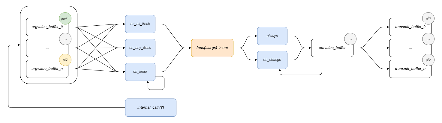
Functions have some state: an input mode (on_timer, on_all_fresh, or on_any_fresh) that defines when it will run, and an output mode (always, or on_change) that defines the conditions under which it will produce new messages.
Pipes can be added to functions: these are message passing specifications that define:
- A route for the message, through OSAP’s network.
- A destination port for the message,
- A list of output indices to transmit (in cases where we want to send i.e. only one or two of the output tuple’s items),
- A list of input indices for the receiver (to map onto it’s function arguments).
3.2.2 PIPES’ Programmer’s Model
3.2.2.1 A Systems Object Model
PIPES implements a Systems Object Model (SOM), which is not unlike the browser’s DOM. It contains:
- A list of OSAP Runtimes, and within each:
- A list of Link Gateways,
- A list of global Pipes Functions that have been instantiated there,
- A list of Pipes Classes that have been instantiated there.
- A list of Links, each of which has:
- A source Runtime and Gateway,
- A destination Runtime and Gateway.
- A list of Pipes, each of which has:
- A source Runtime, Function Name and Class Instance Name (if the function is a member of a class),
- A destination Runtime, Function Name and Class Instance Name
- Output and Input indices, to map the source function’s return tuple items onto the destination function’s arguments.
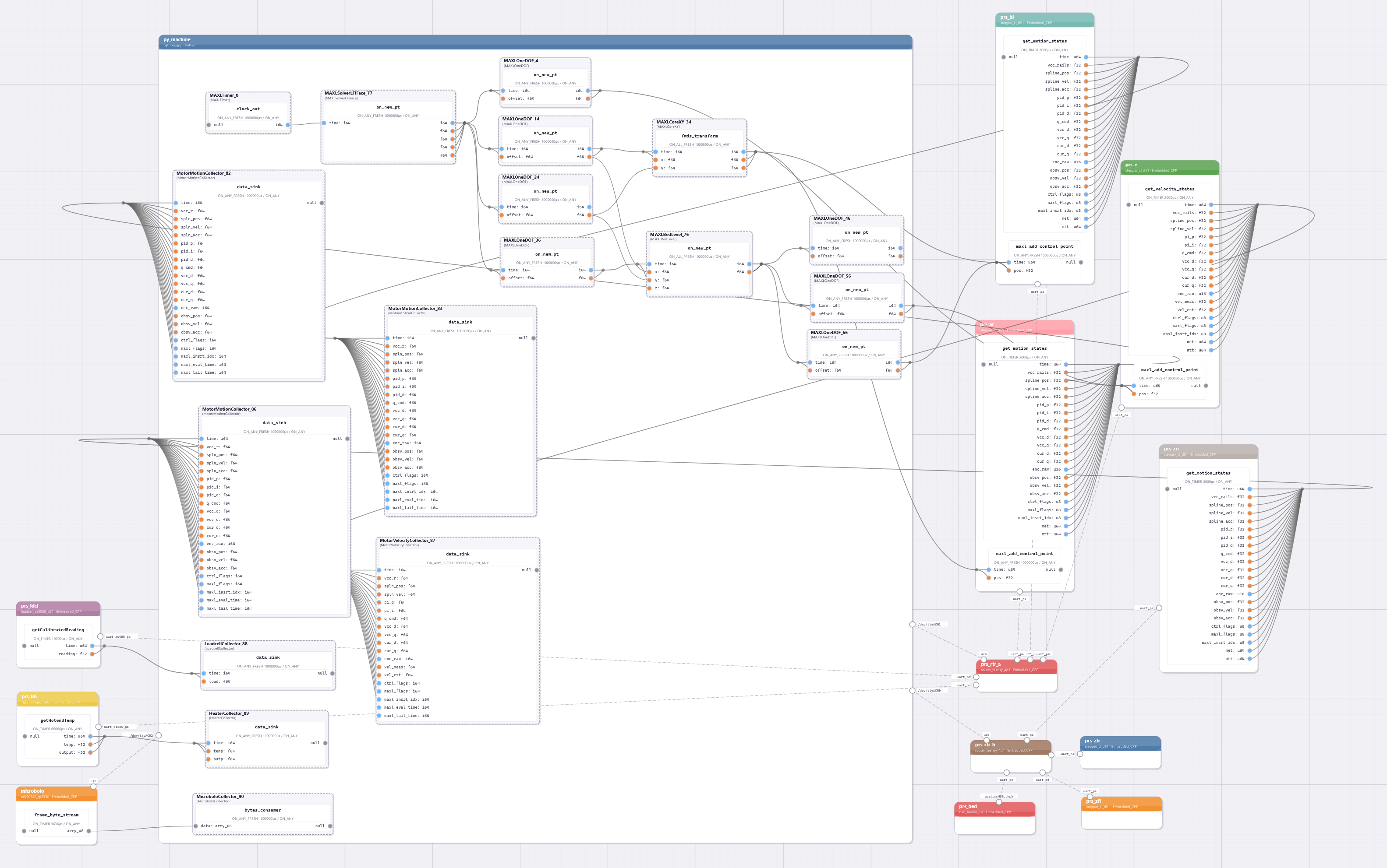
The SOM can be discovered at runtime, starting with network configurations from OSAP, and then adding (by sequentially quering ports within the runtime) the PIPES system description. The interface to this model is provided in software, but the model object itself can be serialized as a .json and rendered, as below.
Interaction with the graph itself only involves making connections between functions, as in Section 3.2.2.3. Classes and functions are each instantiated manually within runtimes, although my Masters’ thesis developed a version where they could be instantiated (and deleted) remotely, allowing for more flexible systems editing.
Interactions with remote functions can also be made via RPC semantics, using proxy classes.
3.2.2.2 Proxies for Remote Runtimes
Devices in the network are exposed to one another in software using proxy classes. This follows the Object Oriented Hardware pattern; they are software classes that can be instantiated in python within one OSAP runtime, and that represent remote hardware: when we make function calls on these classes, they operate that remote functions’ RPC and return the result.
I use the name proxy because I think that it more clearly articulates what the class is: an interface / stand-in object, rather than really “representing” the device itself.
import asyncio
from typing import cast, Tuple, TYPE_CHECKING
from pipes.wrappers.pipes_function_proxy import PipesFunctionProxy

if TYPE_CHECKING:
    from pipes.meta_manager import MetaManager

class AccelLsm6dsv16x:
    def __init__(self, manager: 'MetaManager', runtime_name: str):
        # proxies for global funcs
        self._get_errcode_proxy = PipesFunctionProxy(manager, runtime_name, "global", "get_errcode")
        self._get_data_proxy = PipesFunctionProxy(manager, runtime_name, "global", "get_data")

    async def get_errcode(self) -> int:
        result = await self._get_errcode_proxy()
        return cast(int, result)

    async def get_data(self)-> Tuple[int, float, float, float, float, float, float] :
        """
        returns (stamp: int, ax: float, ay: float, az: float, rx: float, ry: float, rz: float)
        """
        stamp, ax, ay, az, rx, ry, rz = await self._get_data_proxy() #type: ignore
        return cast(int, stamp), cast(float, ax), cast(float, ay), cast(float, az), cast(float, rx), cast(float, ry), cast(float, rz)
These are automatically generated using the data from the routine described in Section 3.2.3, and the templating routine described in Section 3.2.4. They provide a typed interface that can be called directly using RPC semantics, or used as a handle to make connections, as I describe under the next header. Or both: to task machines, we often connect components into dataflow graphs, and then use RPC semantics to activate those graphs.
3.2.2.3 Making Connections
PIPES implements a manager class, which interfaces with the SOM and devices on the network to make changes to the system’s graph configuration. To build Pipes, we use a .connect() function,
# in this case we are piping the timer thru the solver iface,
await manager.connect(machine.timer.clock_out, solver.on_new_pt)
# and solver -> dofs,
await manager.connect(solver.on_new_pt, machine.dof_x.on_new_pt, "0, 1", "0, 1")
await manager.connect(solver.on_new_pt, machine.dof_y.on_new_pt, "0, 2", "0, 1")
await manager.connect(solver.on_new_pt, machine.dof_z.on_new_pt, "0, 3", "0, 1")
await manager.connect(solver.on_new_pt, machine.dof_e.on_new_pt, "0, 4", "0, 1")
These are asynchronous calls because the often require that the manager make requests to functions in remote runtimes. As arguments it takes the proxies for the source and destination functions, and then argument lists (outputs, inputs) to map onto the pipe.
3.2.3 Tools for Module Authorship
Maintaining proxies by hand is tedious and can easily lead to misconfigured systems. One of the most valuable tools that I built during this thesis was the c++ template that automatically turns embedded functions into Pipes functions.
The tool is a compiler macro (BUILD_RPC, name inherited from a pre-dataflow era) that wraps the provided function in a interface class (PipesFunctionIFace) class, which is attached to the OSAP runtime. An example of its use is in Listing 3.3.
// a global function, defined in `main.cpp`

auto get_data(void){
  // read, flip, sendy
  auto tup = std::make_tuple(
    data_stamps[data_reading],
    data_accel[data_reading].xData, data_accel[data_reading].yData, data_accel[data_reading].zData,
    data_gyro[data_reading].xData,  data_gyro[data_reading].yData,  data_gyro[data_reading].zData
  );
  data_reading = data_reading ? 0 : 1;
  return tup;
}

// wrapped with BUILD_RPC to compile a PipesFunctionIFace class.
BUILD_RPC(get_data, "", "stamp, ax, ay, az, rx, ry, rz");
The interface handles message passing between the function and other components in the PIPES system, for example:
- We can query the function for its signature to learn its name, return type, and argument types. This is used to add functions to our SOM 3.2.2.1 and to write proxies 3.2.2.2.
- We can call it remotely (RPC), the other end of that call is normally its proxy, but we can also call it by it’s name (so long as it has been discovered in the SOM, otherwise we must use its network address directly).
- We can configure its input and output modes, and add pipes a-la 3.2.2.3.
@pipes_class_implementer
class MAXLOneDOF:
    def __init__(self, max_vel: float, max_accel: float, output_scalar: float):
        self.max_vel = max_vel
        self.max_accel = max_accel
        self.output_scalar = output_scalar
        self.output_offset = 0.0
        # delta-tee tracker
        self.most_recent_timestamp = -1
        # states tracker
        self.position = 0.0
        self.velocity = 0.0
        self.velocity_target = 0.0
        # for offsets
        self._pos_offset = 0.0
        # stores latest limit states
        self.limit_time = 0
        self.limit_state = False
        # stores pts for history lookup, and blocks for motion
        self.control_points: Deque[MAXLOneDOFControlPoint] = deque(maxlen = 4096)
        self.segments: List[MAXLQueueSegment]
The same tool exists in python, where it is implemented as a function decorator. This is useful on its own for global functions, but more often in python I pull entire classes into PIPES, as in Listing 3.4. Source definitions of python classes will have all of their functions included, except for those which are marked with a leading underscore. All functions that will become Pipes functions must be explicitly typed, for which I use python’s type hinting scheme.
3.2.4 Tools for Systems Assembly
OSAP also includes a network discovery routine (to find, name, and address modular devices). In the last step of this routine, we can query each port’s type_name property, which is a semantic identifier that helps us to link transport and application layers. Pipes Functions are each connected to OSAP with one receiving port, as are class containers. Where we find Functions, we can query for their signatures, and where we find Classes, we query for their signatures, along with a list of their member functions’ port indices.
We use these utilities to assemble the PIPES SOM (3.2.2.1) from the graph that we are currently connected to. This happens at the header of any PIPES / MAXL script, and it is always possible to save the currently loaded SOM to disk as a .json description. We then have the issue of writing proxies. I do this with the templating language jinja (n.d.), with which I transform device and function definitions into proxy classes like the one shown in Listing 3.1.
To bootstrap a programming entry point, I also wrote a utility that generates a starter script for the system. Using all of this, we can automatically build programmable interfaces for sets of modular hardware.
3.3 MAXL: Dataflow Motion Control
Modular Acceleration planning and eXecution Library
The development of MAXL is motivated by two main goals 3.1.4. The first is to build motion controllers that expose a rich interface to their velocity controllers (Section 5.2.1 and Section 5.6) so that we can better understand real machine behaviour. The second is to develop motion control as a system of modules that can be easily reconfigured for a variety of machines.
3.3.1 MAXL’s Operating Principle
MAXL works by sequentially transmitting trajectory segments between dataflow blocks. Most of these blocks (Section 3.3.3) are written in python as PIPES classes, and trajectory interpolators are written in c++ as PIPES functions. I originally developed the basic premise in (Read, Peek, and Gershenfeld 2023): by encoding trajectories as some set of interpolatable functions of time, we can simplify trajectory execution (at any time, firmwares can query trajectories to pick an appropriate action, like update a servo’s target position or trigger a switch or sensor) and make the reconstruction of machine motion more straightforward computationally.
In that earlier paper, I developed a few types of interpolatable functions: linear trapezoid segments to encode motion event tracks, which simply change value at set times and can be used as triggers for sensors or control setpoints for lower level systems. In this implementation, I use only one: cubic basis splines (3.3.2).
The key bit of the architecture in that paper which is extended here is that trajectory authors and interpolators both share a time based representation for the trajectory, which is written after velocity scalings are applied by controllers.

This provides a framework for flexibly adding devices to machine systems that must interact tightly with (or synchronize to) its real-time motion. Machines spend a lot of time changing velocity; trajectories encoded in GCodes cannot be interpolated in time because they do not encode this velocity scaling - that is done beneath GCodes. As I will discuss elsewhere, this causes issues for machine builders and process researchers - the instructions that we send to the machine are modified, and we cannot ascertain what was actually done when our instructions ran. Of course this requires that devices in the system share a time basis, here we have OSAP’s synchronization service 2.2.4.2 for that purpose.
In this section I extend that concept in a dataflow configuration. This allows us to reconfigure motion control systems by re-wiring graph connections rather than re-writing software, and helps us to include motion control as a component of a larger machine control system.
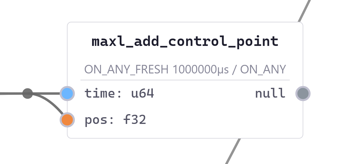
The premise in MAXL is that:
- Device clocks are synchronized.
- Trajectories tick along at a fixed interval, which is set by the Timer block 3.3.3.1. It outputs a new time stamp once in every interval.
- Other blocks (a set of which are explained in Section 3.3.3) trigger on these timestamps, using whichever logic they would like to implement to generate a new output value at that time. In many cases, blocks add, multiply, or otherwise combine their contributions to that value with inputs that were generated by other blocks. Values are output alongside time-stamps, making for time-series sets of values of various shape. Besides operating or modifying these values, maxl blocks can also interpolate them, i.e. as basis splines, to produce outputs that are useful in their local environment (i.e. as position or velocity targets in a servo).
Because components are distributed across networks, we need a strategy to ensure that the time between trajectory generation in software and interpolation in hardware is no shorter than the maximum interval that it may take for the trajectory point to reach the interpolator. I explain how this is managed in Section 3.3.3.1.
3.3.2 Synchronized Basis Splines
To describe motion in time, MAXL uses a cubic basis spline interpolation (often just called a B-spline) with control points (aka knots) at fixed time intervals. Basis splines are often used to representation motion because they have well defined and smooth derivatives for velocity and acceleration, with step functions in jerk (Holmer 2022). This matches particularely well to inertial systems controlled by electric motors because they have the same order; as discussed in Section 5.3.1, our actuators cannot instantaneously change the amount of torque (acceleration) they are exerting, since it takes time for an applied voltage on the motor stator to develop into current. This means that electric motors cannot instantaneously change accelerations, although they can make instananeous changes to the rate of change in acceleration (i.e. voltage, jerk).
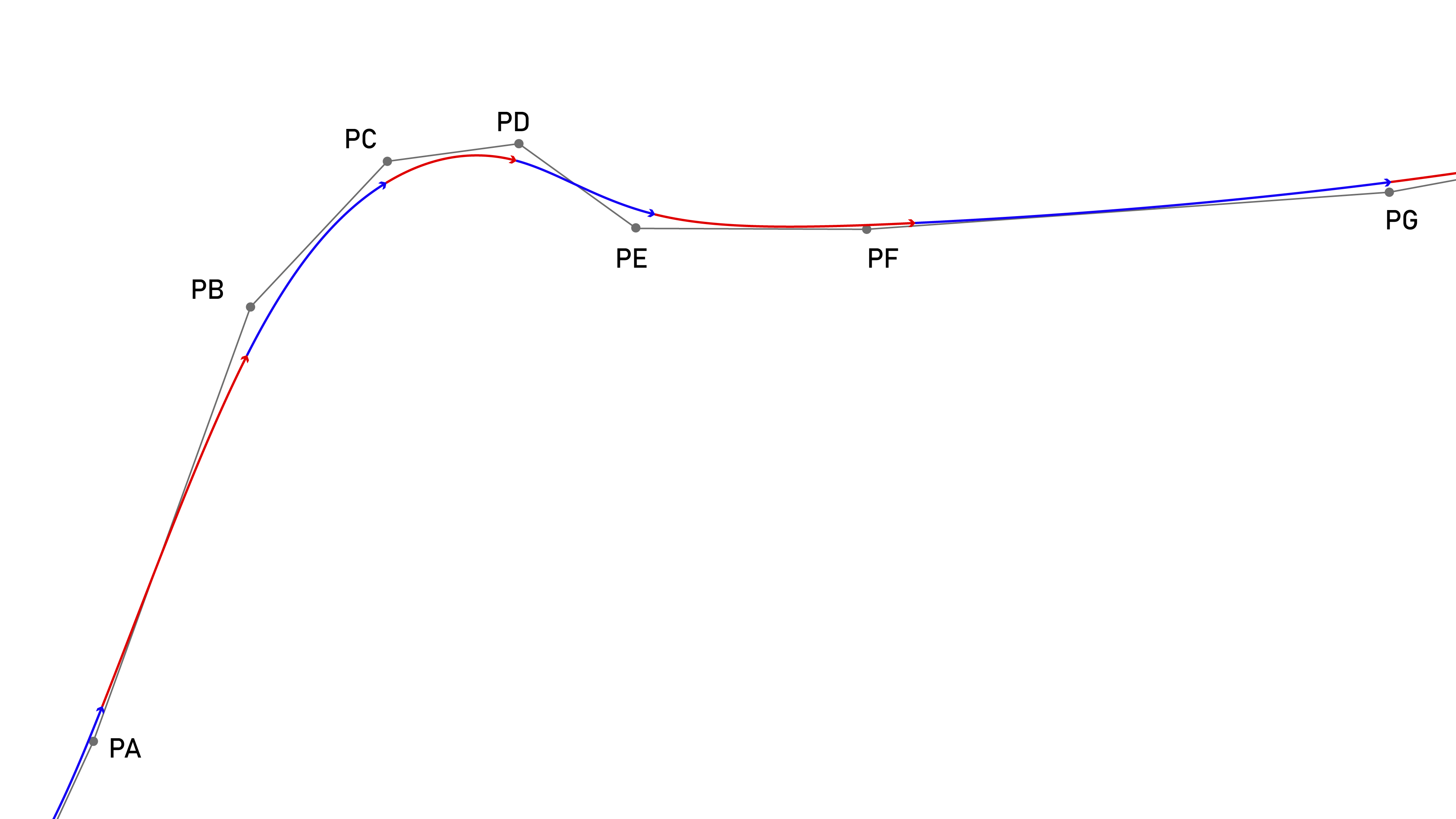
\[ P(t) = \begin{bmatrix}1 & t & t^2 & t^3 \end{bmatrix}\frac{1}{6} \begin{bmatrix} 1 & 4 & 1 & 0 \\ -3 & 0 & 3 & 0 \\ 3 & -6 & 3 & 0 \\ -1 & 3 & -3 & 1 \\ \end{bmatrix} \begin{bmatrix} P0 \\ P1 \\ P2 \\ P3 \\ \end{bmatrix} \tag{3.1}\]
Equation 3.1 is the cubic basis-spline form that MAXL uses. \(t\) spans a fixed interval, and the interval is set at some integer value of microseconds that is a power of two, between 256us and 16384us. Using these intervals means that the spline can more rapidly be evaluated using fixed point arithmetic in embedded devices. Basis splines have the helpful property that we can always add new points to the end of a stream, meaning that at each interval we only need to stream one new position (whereas i.e. a linear segment of similar length would require much more information).
3.3.3 MAXL Blocks
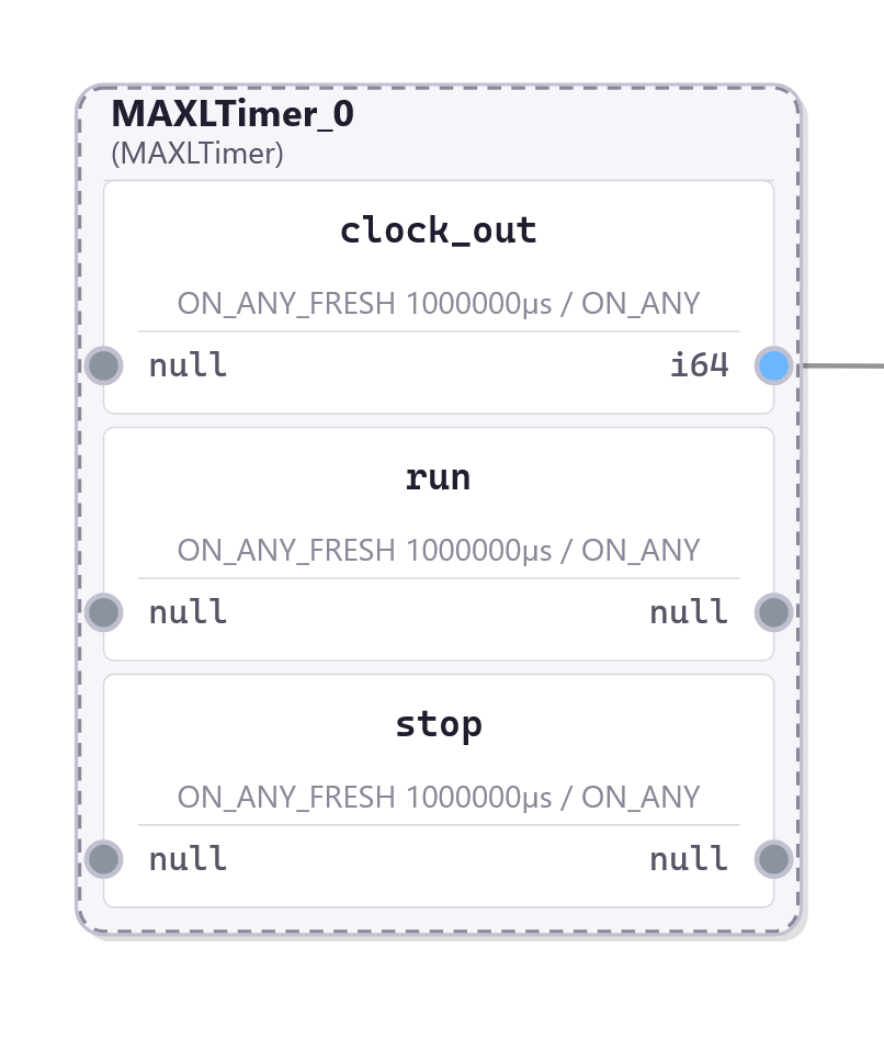
3.3.3.1 Timer
The timer outputs one new timestamp within each (fixed) interval, where the interval configured as some number of microseconds. These ticks then trigger downstream blocks to produce new outputs. Transmitting trajectory components at fixed time intervals is valueable for two main reasons:
- It means that blocks which operate as integrators can do so using a repeating \(\Delta t\)
- It makes for deterministic network loading, whereas i.e. transmission of line segments can lead to bursts of network traffic when a machine transitions from a long segment into sections of high geometric complexity.
To maintain that trajectory components arrive at interpolators in time for their evaluation, time stamps generated here have some amount of advance, configured as a number of ticks into the future. For example if our interval is \(1024 \mu s\) and advance=16, the timer will generate a timestamp for \(t = 16384 \mu s\) at \(t=100000 \mu s\), effectively leading the system clock by those \(16384 \mu s\).
3.3.3.2 OneDOF
The OneDOF is a utility for controlling single degrees of freedom (DOFs). It is used in-line with axes of motion to add general purpose motion functionality to those axes. It contains a single-segment trapezoid generator that can be used to move DOFs smoothly from point to point, and a velocity control mode that applies acceleration control.
It also implements a simple homing routine, where the limit signal is exposed as a pipe input, meaning that we can source home signals from any module in the system. For example to level 3D printer beds, I use a comparator output from the loadcell sensor to trigger this “switch” in combination with a OneDOF block that is chained into all three z-motors.
3.3.3.3 Chirp Generator
The chirp generator is another simple motion utility that I use in the generation of preliminary motion models. It writes chirp time-series using scipy (Virtanen et al. 2020) and interpolates through them to produce outputs.
3.3.3.4 Trapezoidal Planner
This is a planner that ingests line segments, queues them, and plans velocities across them as described in Section 5.2.1. In systems that use this planner, it is typically the second block in the dataflow - the first being the timer.
3.3.3.5 Optimizer Interface
The optimizers developed for velocity planning in this thesis are integrated within machine systems using MAXL via an interface block that I describe in Section 5.6.2.
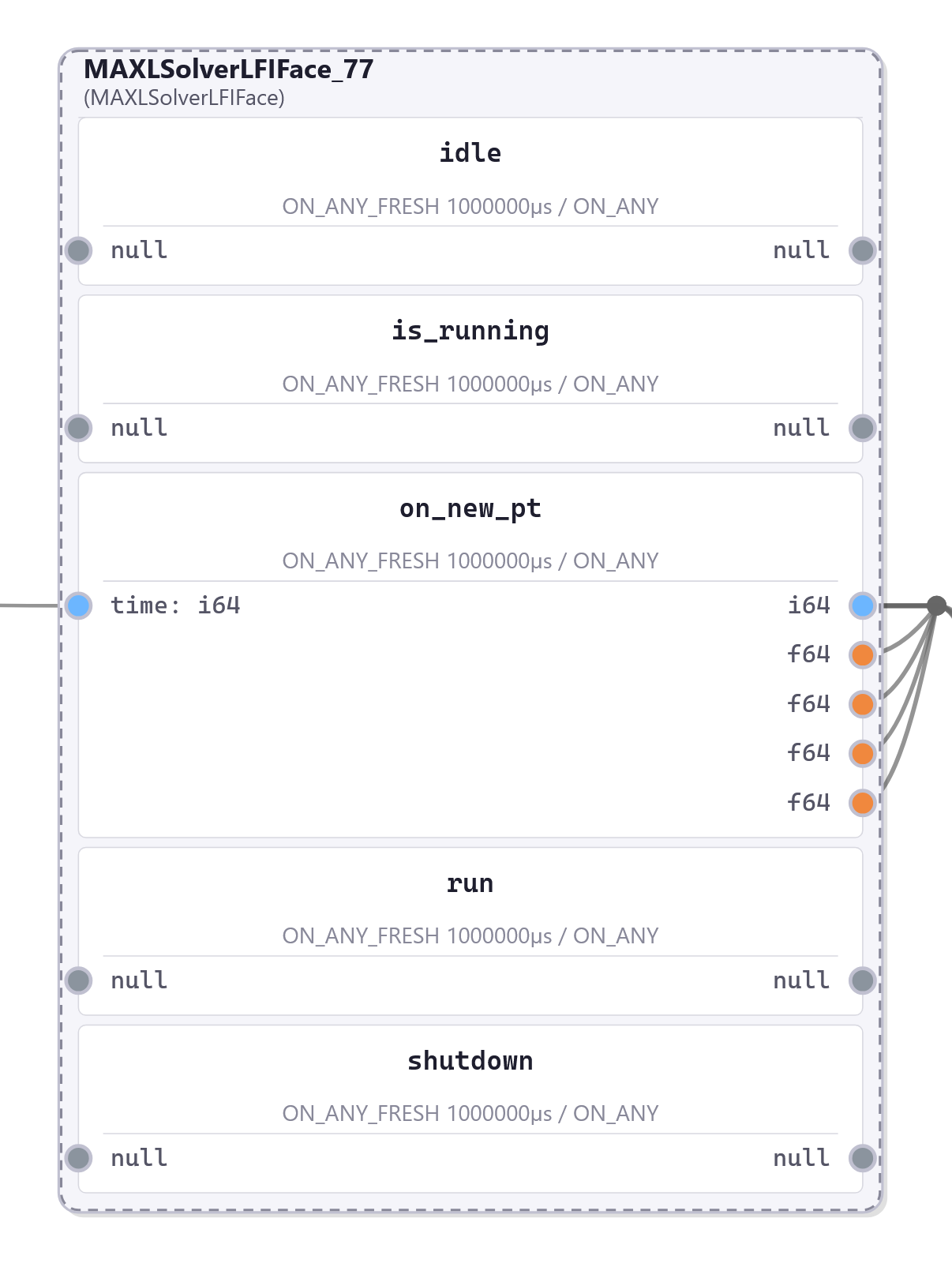
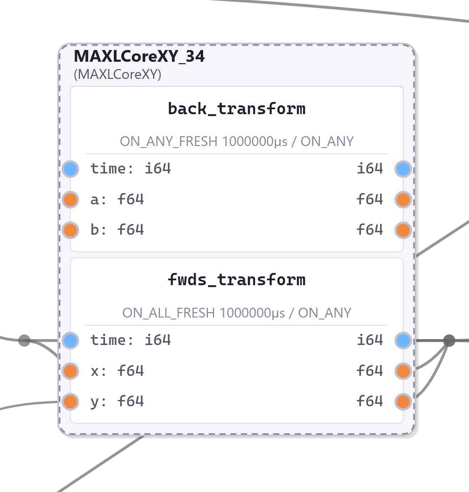
3.3.3.6 CoreXY Kinematics
Implements CoreXY (I. Moyer 2024) kinematics.
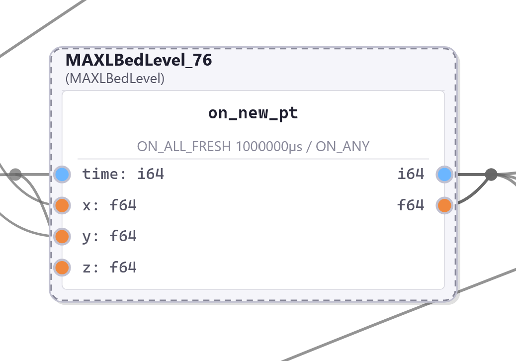
3.3.3.7 Bed Level Corrector
The bed level corrector is used in-line with z-axis motion, and also reads xy states, using those to interpolate through a bed correction map and add the offset correction to the stream of z points.
3.3.3.8 Spline Interpolator
Normally the terminal end of a MAXL system, the spline interpolator follows the logic outlined in Section 3.3.2 to generate interpolated \(p(t), v(t), a(t)\) and \(j(t)\) values. In this thesis, these are used by the motor controller in Section 5.4 as position and velocity control inputs.
3.4 Evaluating PIPES and MAXL
3.4.1 Visibility of As-Planned Velocities
- Most velocity planners are in firmware, beneath GCode, so we cannot see the results of their internal operation. Relocating planners into software has the effect that we can now easily visualize the results of our machines’ velocity planners’ actions on their target trajectories.
- MAXL and PIPES go to some length to remove velocity controllers from firmware, relocating them as software objects. One of the primary benefits of this is the simple utility of being able to inspect these controllers’ outputs and easily modify them. Their configurations and those configurations’ relationship to our machine hardware and our target path geometries can combine to produce interesting results.
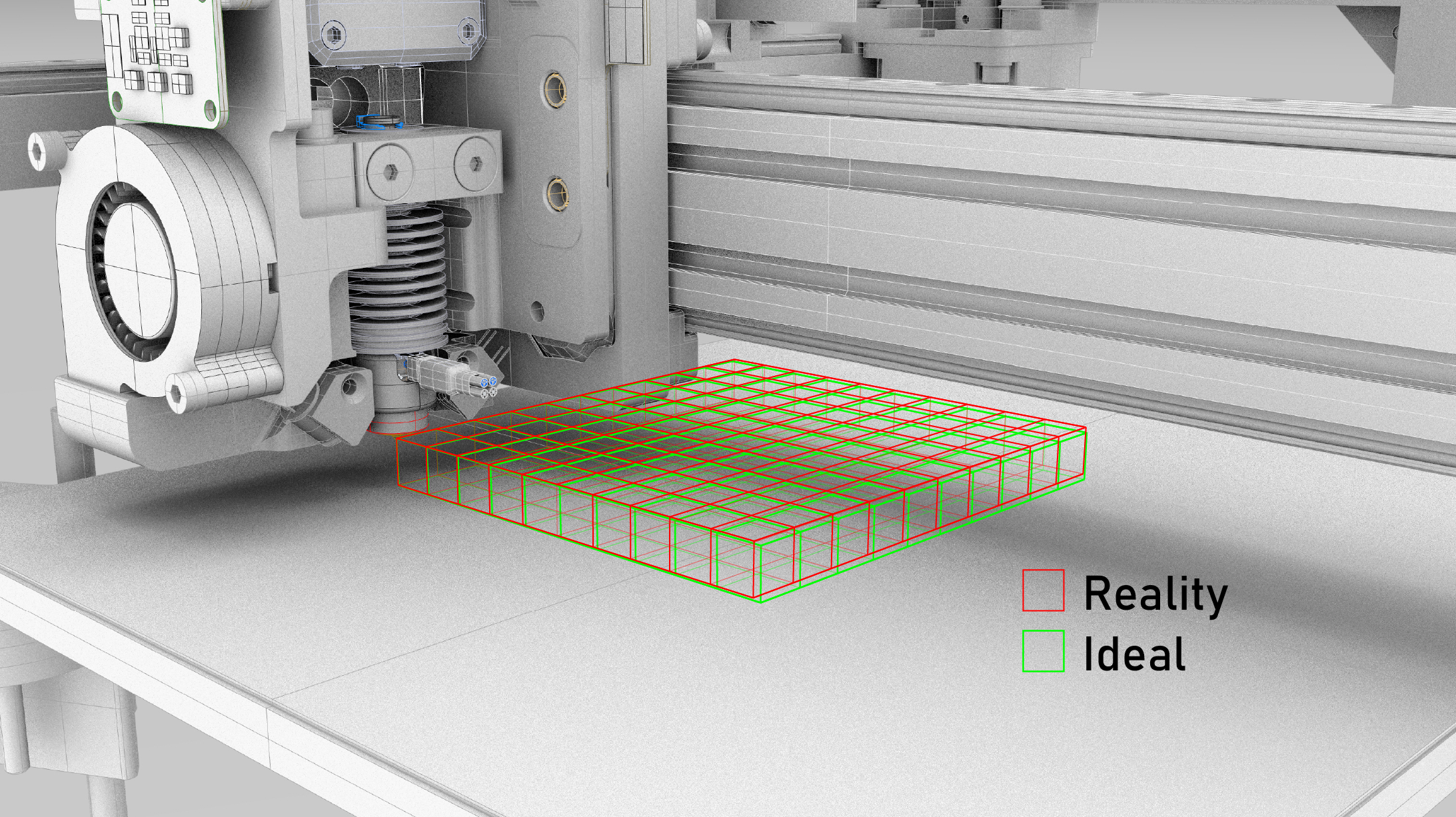
For the first example of this, see Figure 1.8 from the introduction, where I show that in some parts of path- and machine-parameter space, the feedrates that GCodes specify may never be reached when they are actually run on hardware.
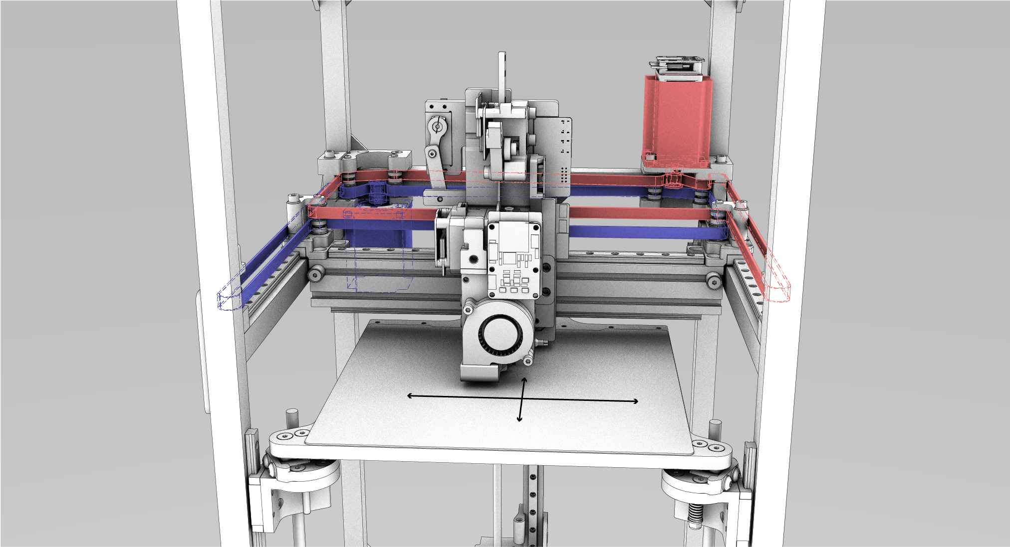
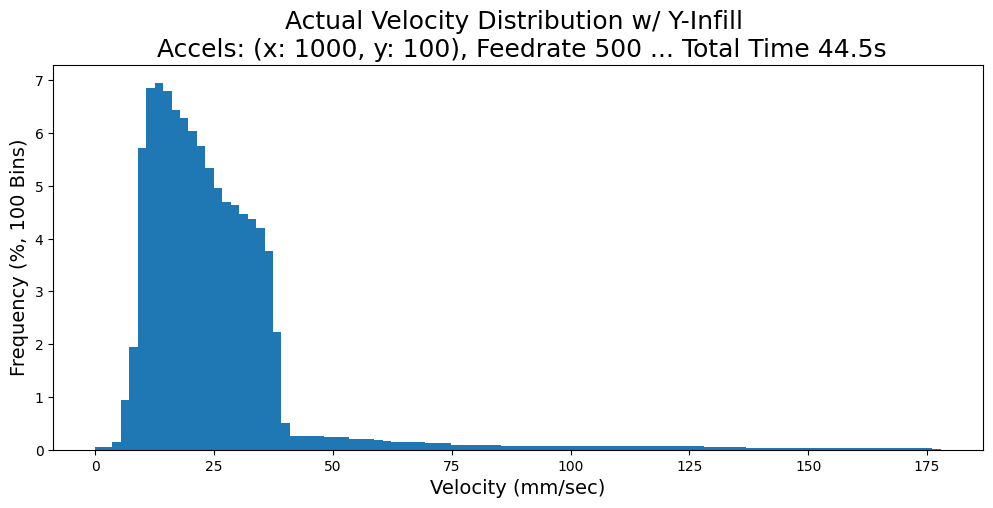
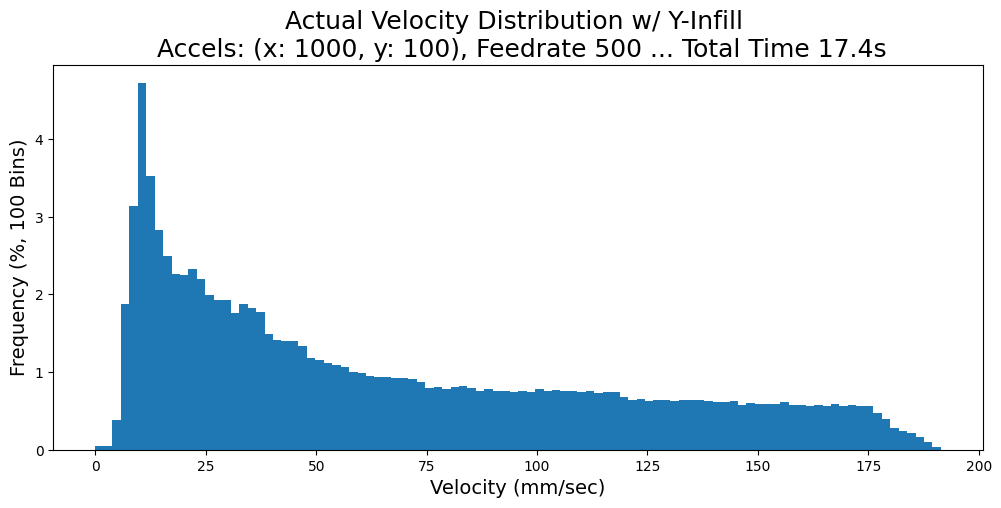
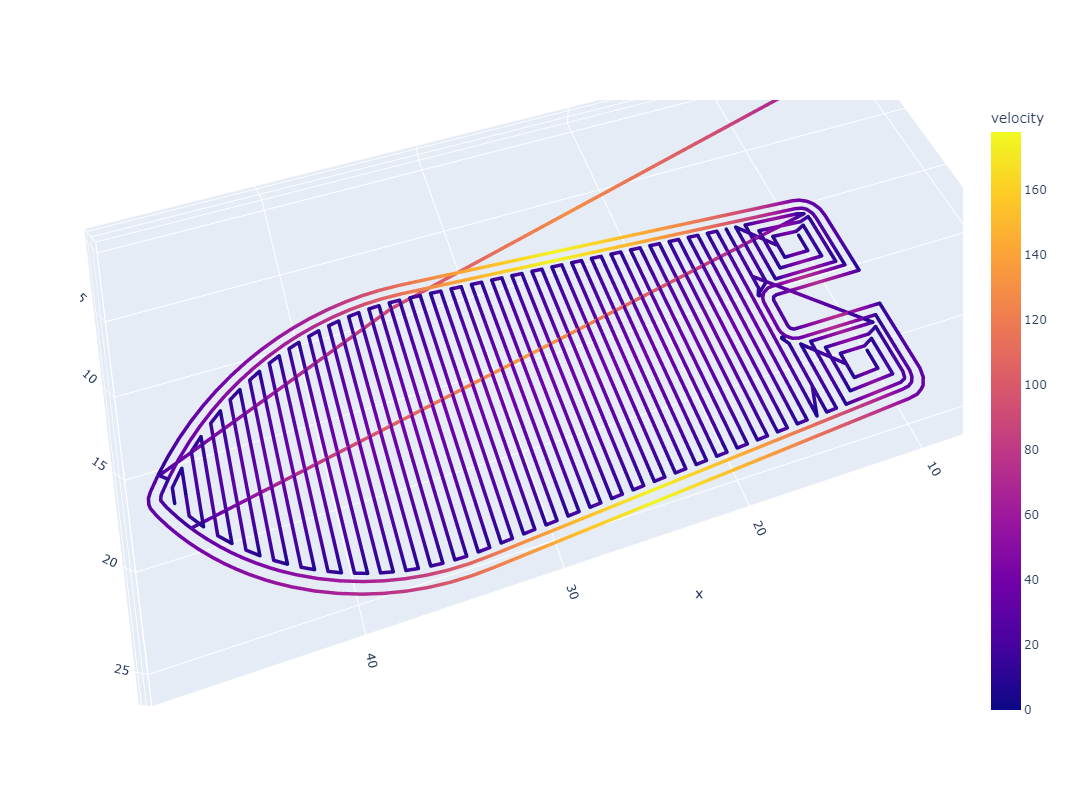
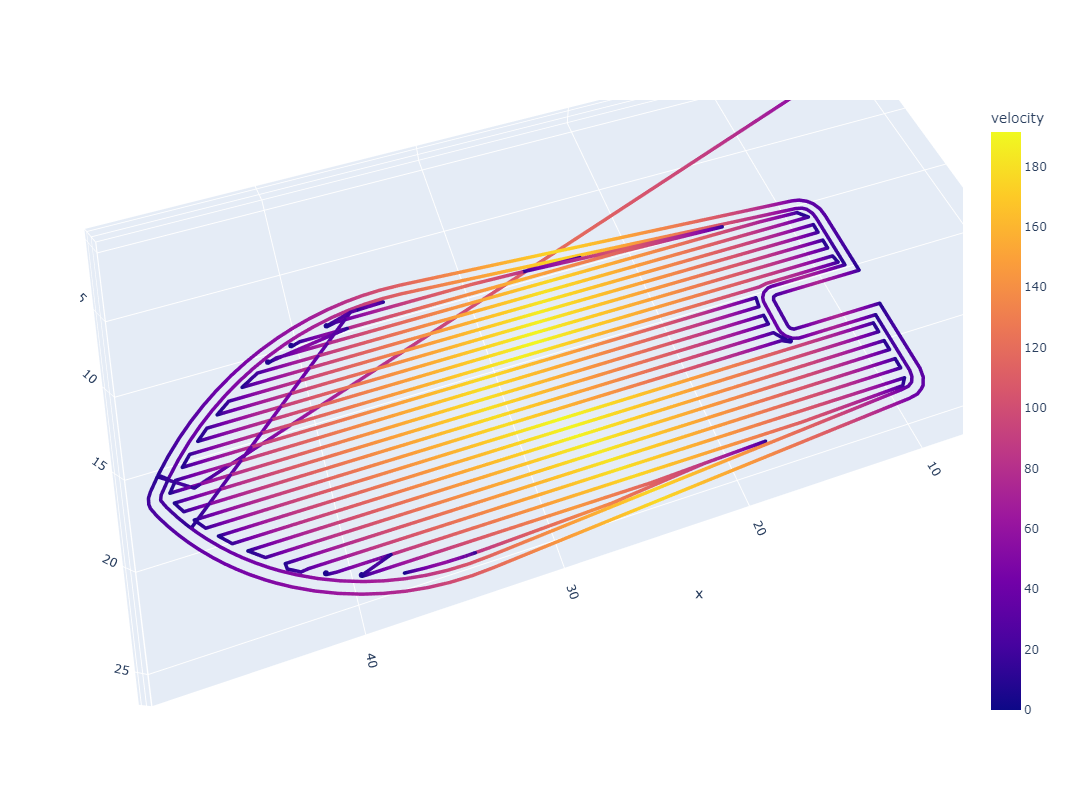
For another example, consider CoreXY ((I. Moyer 2024), more detail in 3.3.3.6): machines with this layout have highly anisotropic dynamics. Both motors work together to move the machine in X and in Y, but the moving mass in X (just the end effector) is significantly lower than that in Y (which includes the end effector along with the y-beam). In the figure below, I show outputs using a trapezoidal solver which deploys 10x more acceleration in the X axis than in the Y; we can see that changes to path geometry (like aligning repeated, long line segments to the motion systems’ anisotropy) can significantly change outcomes (like total processing time, and actual processing feedrates).
In Section 7.4.1, I show how this result from MAXL’s structure enables the development of a simple tool for visualizing chip load deviation in CNC machining toolpaths. In that context, this knowledge can be invaluable before a path plan is run on a machine because significant chip load deviation can lead to chip welding (rather than cutting).
3.4.2 Time Synchronized Sensing and Data Collection
Using a time basis for trajectory representation leads to many other outputs in this thesis, because it allows us to combine sensor data with motion data. I show how this capability is used for model building in:
- Fitting kinematic models, Section 5.5.2
- Improving kinematic models using data generated during machine operation, Section 5.7.3
- Fitting dynamic extruder parameters, Section 6.5.4
- Fitting coupling terms between extruder motors and melt flow models, Section 6.6
In each of those cases, I use motion controller inputs to drive systems while collecting time-series data of motion states alongside sensor data, which are then used to fit (or update) models. I also show how this capability is used to evaluate motion systems:
- To evaluate the quality of kinematic models, Section 5.7.2
- To generate new insights from 3D printer data that combines sensor, motion, and solver states, Section 6.11.2
- To make cutting force estimates, combining kinematic models, motor models, motor data, and trajectory data, Section 7.5.4
3.4.3 Reconfiguration of Systems for Model-Building or Model Deployment
Same hardware, new software.
I use different controller configurations in scripts that I use to develop model-fit data than those where I use machines to make parts. For example the 3D printers in Chapter 6 each has four total configurations:
- To fit flow models, where just the extruder system is activated. In this case, the motion control graph consists only of a Timer, a Chirp, and a OneDOF block (and the extruder motor). All other operation of the system (setting and waiting for nozzle temperatures) is done with RPCs, and data is collected with a series of Pipes: from the loadcell, the extruder motor, and the nozzle heater.
- To fit motion models, two configurations:
- To run chirp tests on the XY/AB kinematic system,
- To run chirp tests through the Z motors.
- To operate the machine: using the full gamut of devices and adding the printer’s solver interface.
Configurations of the CNC mill from Chapter 7 are similar:
- To fit motion models, three configurations - one to test each axis.
- To run the machine, two configurations: one of which uses a trapezoidal planner, the other uses the optimization based solver from Section 5.6.
3.4.4 Reconfiguration of Modules for Machine-Building
Same software, new harware.
The thesis is filled with examples also of the same hardware appearing in different machines. The 3D printer and milling machine above are the clearest example of this.
The OneDOF module is repeated by far the most often in different systems and configurations, which makes sense given that most machines have at least… one degree of freedom. Its utility in quickly adding simple control interfaces for “the rest” of machine control (i.e. the jogging, the homing, etc) is invaluable, and means that we don’t have to add that complexity into other modules like the trapezoidal planner or solver.
This has a limit though, for example the velocity planners for the 3D printer and CNC mill are each unique: they are “reconfigured” for each machine by re-writing software. In kinematics this is true as well, we cannot compose arbitrary mathematics with the existing set of MAXL blocks, and need a new module each time we encounter some new arrangement of axes.
3.4.5 Expressing Kinematics
A sub-task in the reconfiguration of modules for machine-building involves capturing different kinematic configurations. With MAXL, I try to do this with graph reconfiguration… Examples above already show a 3D Printer with CoreXY kinematics and a bed leveling correction tool, as well as a simple cartesian machine. Can we do more?
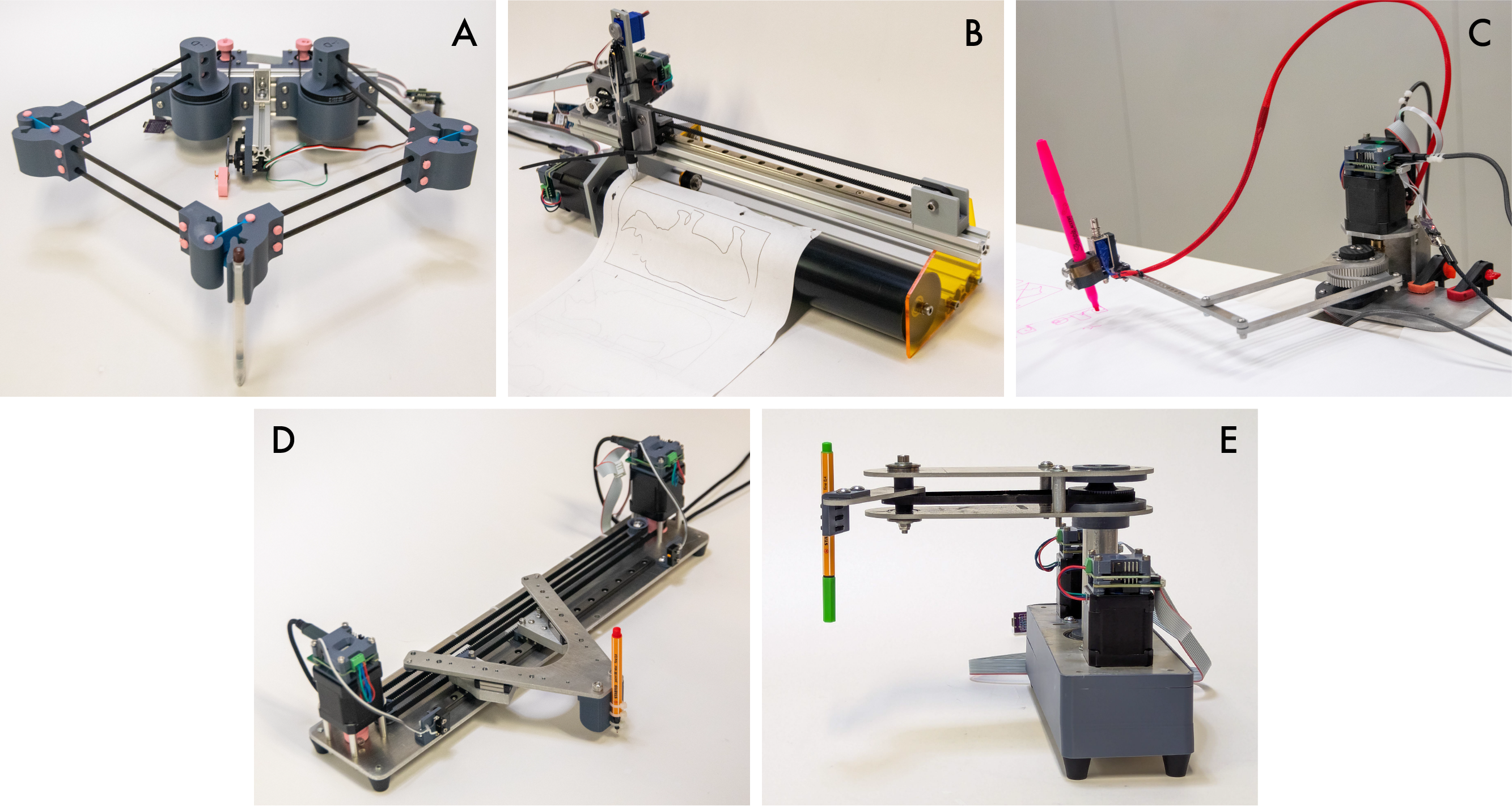
- We ran a workshop at the CBA where participants developed drawing machines. I participated as a machine control enabler, and used MAXL (it’s trapezoid planner and overall structure) to quickly develop controllers and kinematics models for each of these machines.
- That involved working with machine designers to describe their kinematics as functions that map tool-tip positions to motor positions (IK), and then authoring those together as python functions. Those were then written as MAXL blocks, and connected to hardware with PIPES.
- We successfully drew .svg’s with each machine, showing re-use of software modules across variable hardware.
3.4.6 AdHoc Systems
3.4.6.1 CNC Xylophone
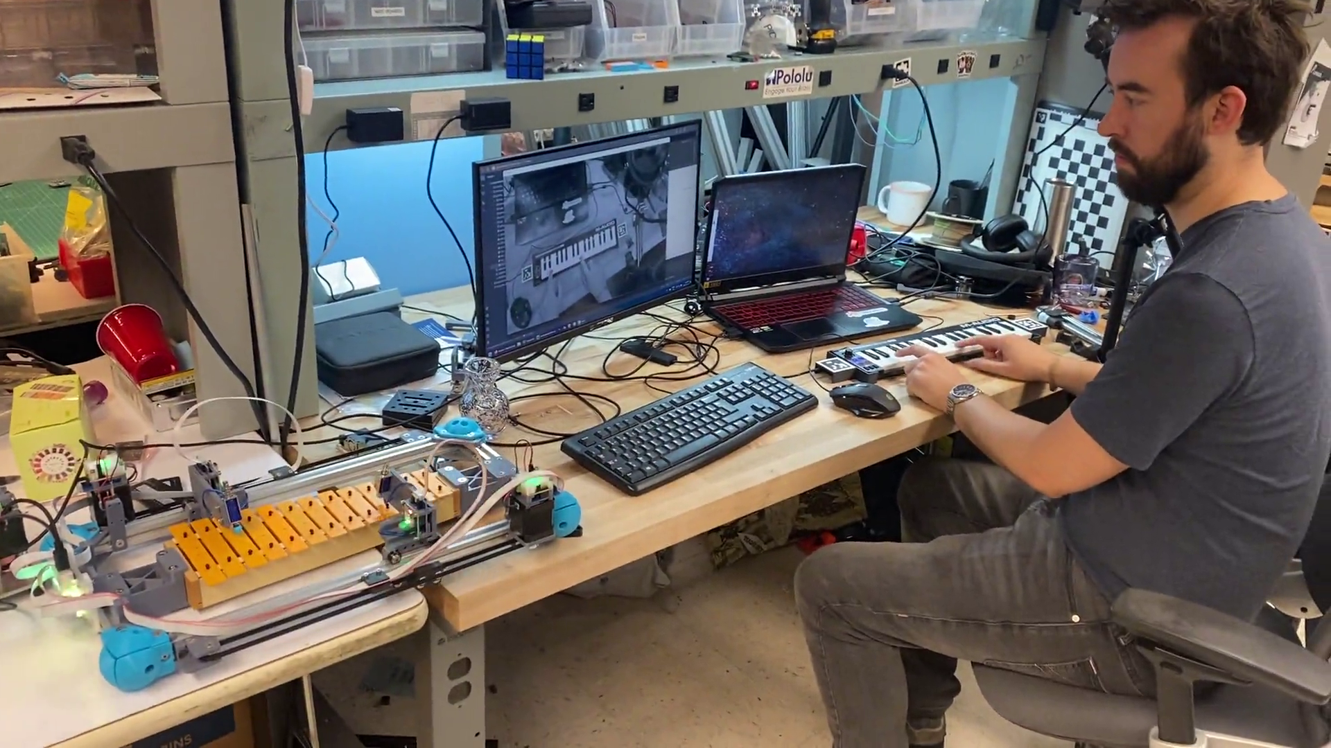
As a playful machine demonstration for Fab Class (Gershenfeld, n.d.), I worked with Quentin Bolsee and Jens Dyvik to build a computer controlled xylophone. It is controlled with two OneDOF blocks and two open loop stepper controllers. The hammers are solenoids that are activated using RPC calls.
  async def handle_echo(reader, writer):
      print("Connected")

      stop_requested = False
      while True:
          data = await reader.read(100)
          if not data:
              break

          msg = pickle.loads(data)
          if msg.get("running", False):
              stop_requested = True
              break

          reply = {"ACK": True}
          writer.write(pickle.dumps(reply))
          await writer.drain()

          if "hit" in msg and msg["hit"]:
              using_a = True
              if "note" in msg:
                  p = note_to_pos(msg["note"])
                  pa = dof_a.get_position()
                  pb = dof_b.get_position()
                  if abs(pa-p) < abs(pb - p):
                      await dof_a.goto_pos_and_await(p)
                      using_a = True
                  else:
                      await dof_b.goto_pos_and_await(p)
                      using_a = False
              if using_a:
                  await fet_a.pulse_gate(0.85, 6)
              else:
                  await fet_b.pulse_gate(0.85, 6)
          else:
              if "note" in msg:
                  p = note_to_pos(msg["note"])
                  pa = dof_a.get_position()
                  pb = dof_b.get_position()
                  if abs(pa-p) < abs(pb - p):
                      await dof_a.goto_pos(p)
                  else:
                      await dof_b.goto_pos(p)

      writer.close()
      print("Close the connection")
      await writer.wait_closed()
      print("done")
      if stop_requested:
          flag_running.set()
Quentin added a computer vision system that detects a user’s fingers above piano keys, and listens to MiDi input over USB. This then generates instructions for the machine interactively. Rather than rebuild build that system in PIPES, he simply modified my xylophone control script to open a socket into his process.
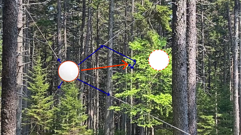
3.4.6.2 The Blair Winch Project
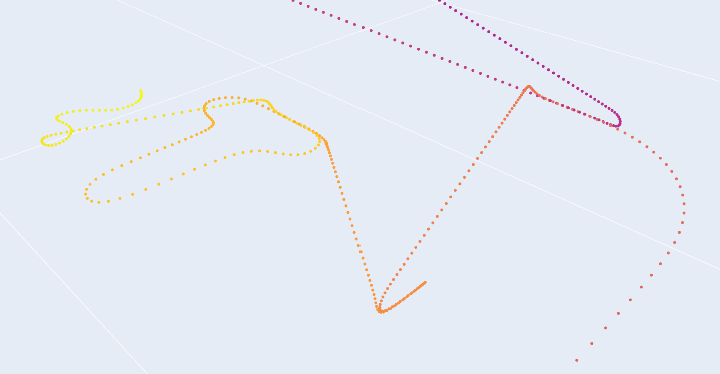
Last summer, I made a small piece of machine art that I called the blair winch project,(2025) which suspends an orb of light amongst some trees in the woods in Maine (at Haystack (Rutter and Gershenfeld 2025)).

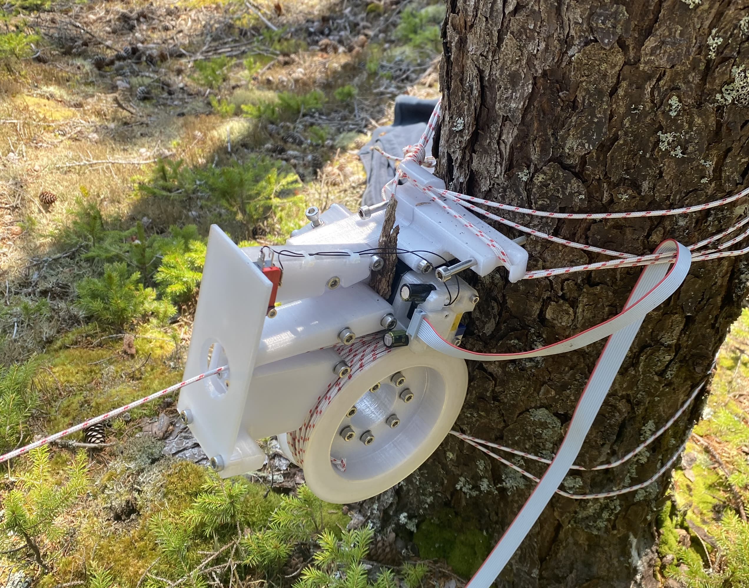
For this project, I used direct control of the motors’ current to move the orb; rather than using MAXL blocks, I simply wrote a feedback controller in python that measured cable lengths (via RPC calls to get motor positions), computed torques that would apply the tensions that should move the orb into the desired position, and then sent those torque requests back to motors (with another set of RPC calls to Pipes functions).
3.4.7 Workflow Capture
On this front we fall on our face: many components in our workflows are i.e. modelling notebooks, where we are copy-pasting parameters about, and requiring file i-o to work, i.e. in Section 6.3 and in many of the modelling steps: systems are run to produce data, which is then saved to disk, and opened in another script for analysis and fitting. The thesis describes the goal of smoothly moving between high- and low-levels, but in these workflows (despite having success in developing representations that are valuable throughout), we still struggle to assemble the use and development of those workflows.
3.5 Discussion
3.5.1 Evaluating against Design Goals
- In Section 3.4.1, I showed how software-defined machine controllers allow us to collect as-optimized velocity trajectories or more complex states from optimization based motion solvers. Combining this capability with time-synchronized data collection over PIPES and OSAP 3.4.2 lets us inspect motion control states alongside sensor readings, which in turn helps us to build predictive systems models.
- Section 3.4.3 shows how PIPES / MAXL are used to re-configure and then task hardware for the purposes of model building and model deployment. (Same hardware, new software).
- Section 3.4.4 shows how PIPES / MAXL can be used to redeploy software and hardware modules in new machine configurations. (Same software, new hardware).
3.5.2 Replacing File-IO Workflows with Systems
I mentioned in Section 3.4.7 that PIPES/MAXL fails to capture complete machine workflows, which I posed as a challenge in the introduction 1.3.
The overwhelming challenge here is to describe types and data structures, and serialize them. This is basically what file-io is anyways, except that they are stored to disk rather than piped.
The other challenge is of inclusion - our system requires that each software module present itself in an OSAP runtime. Limitations there prevent us from quickly doing so, but simple interface classes may be an answer.
The last is simply… engineering labour. Even with the tools developed here (and discussed under the next heading), there is a lot of code to write if we want to accomplish this goal.
3.5.3 Programming Overhead
In Section 3.1.4 I asked: “is the overhead for the systems programmer minimal? What about the module authors?“
In Section 3.2.3 and then Section 3.2.4, I show how PIPES and OSAP enable us to rapidly integrate new firmwares into machine systems. Comparing this to some common practice in the development of workflows that cross between i.e. python scripts and firmware, we can see that our tools make some progress.
- Functions are cleanly represented and typed across systems, and no manual authorship of i.e. “newline-delimited string parsers” is required (2024).
- Systems can be automatically collected and interfaces automatically written, providing boilerplate code templates for machine developers.
3.5.4 Out of Band Use
In Section 3.1.4 I mentioned that “4. Where the architecture fails to capture our intended system, is it easy enough to circumvent or modify it?
The xylophone is a good example of this. Because the xylophone’s controller is a python script, Quentin can easily write a socket that connects to it. Eschewing PIPES, he simply wrote his own interface on top. This is easier to do with a software defined machine because the script that runs the hardware is easier to modify than i.e. a firmware-based controller may be (requiring that code be recompiled and re-flashed onto hardware). The xylophone is also not a project we would have embarked on if we needed to design a new PCB and write a new firmware in order to complete it.
The blair winch project is another example. Rather than trying to articulate the controller as a MAXL block, and have motors follow trajectories, I simply update torque requests to motors in soft real-time, which is acceptable for this application. In fact, that system doesn’t use any graph configuration at all (same with i.e. the motor modeller), the RPCs are enough. This is OK because the system is quite slow overall: the network is much faster.
3.5.5 GCode, Timing and the Partitioning Problem
Perhaps the most important point / caveat to this system is related to Section 3.1.1 and what is perhaps the main reason that GCode still exists, which comes back to design of networked control systems.
Our system allows machine builders to quickly modify data flows in a network. However, it cannot guarantee that these flows will be possible: it is easy to request a transmission interval from a device that will saturate a network link. This is one reason why i.e. state-of-the-art controllers (3.1.3.2) don’t allow for reconfiguration on their networks: those loops and networks are carefully designed such that performance remains deterministic.
This performance-based architectural constraint leads to the representations we use: i.e. these approaches are basically why we have gcode: this middle layer can’t provide arbitrary interfaces because it needs to be un-editable. From this viewpoint, GCode (rather than a pollable controller API), has the advantage that it cannot be queried repeatedly or modified.
In Section 2.4.3, I discuss how future improvements to OSAP’s timing layers could enable us to feed network performance measurements back to systems assemblers. Combined with PIPES, where data loads generated by the graph can be calculated (where we use functions on timers, and know the list of types being transmitted in each), we could build tools that show which network links in a graph are overloaded. This might help to add flexibility in networks while still maintaining performance guarantess.
3.6 Future Work
3.6.1 Improving PIPES Types
The type system in PIPES, which is limited to a simple set of types and tuples (no named data structures or multi-dimensional arrays) presented some real limits to systems development in this thesis, and should be improved.
3.6.2 PIPES Manager in Firmware
Embedded PIPES devices are currently limited in their flexibility. While I have assembled systems that can do these things before, we should bring the same back to PIPES.
- Load and delete functional blocks, in firmwares, at runtime,
- Remotely operate other firmwares and devices, from within firmwares (i.e. outfit the embedded PIPES build with our scripting and systems assembly interface).
The first of these requires some amount of runtime resource management in embedded, which brings memory management requirements and can be dangerous in embedded systems. The second requires (or is difficult to do without) an async API, which is difficult to build in C++, but straightforward in Rust.
3.6.3 Remote Editing of Function Source Code
Whereas it is possible to author many of the modules we will want to have available in each of our devices, the current strategy (where they are loaded into devices a-priori and then assembled) has two major drawbacks.
- Remote functions become black boxes. Especially because machine design and control mixes nomenclature from multiple domains, it is difficult to ascertain what exactly a functional block actually does from its name and input/output types alone (although types are extremely valueable here). If we could pull source code from these functions as well (or at least, good documentation), much of this confusion could be avoided.
- We can never completely anticipate what functional blocks we will want to build. A great programming point I once heard was something like “my favourite part of dataflow programming systems is the little block I can add that I can write code inside of” - this rings true.
In python- and javascript-based PIPES / OSAP runtimes, this shouldn’t be too much of a challenge, and micropython may be a good way to implement the same in embedded devices, although that has its own drawbacks. I expect that a true computer scientist type of magician could figure out how to spot-compile functions for a microcontroller and build a kind of partial bootloader to inject new functions on the fly: it may also be the case that a building a network bootloader handle in OSAP is enough, and where we want to add new blocks we simply recompile the device’s entire firmware, reload it, and reset it.
In any case, the value in being able to completely describe a distributed system in this manner is sure to be of major importance if we go towards trying to build robust, safe, and verifiable systems in an architecture like this.
3.6.4 Developing a Visual Graph Interface
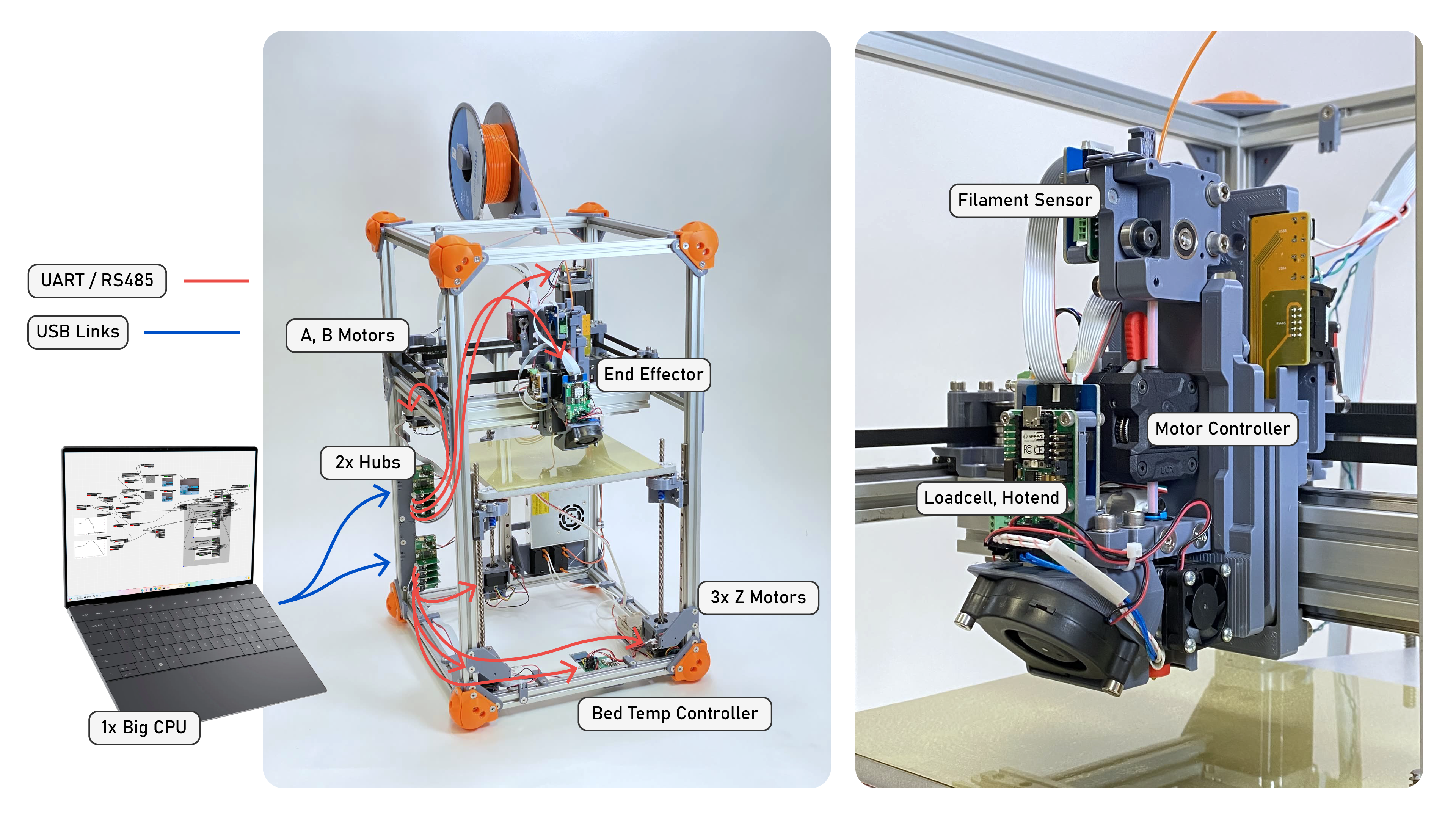
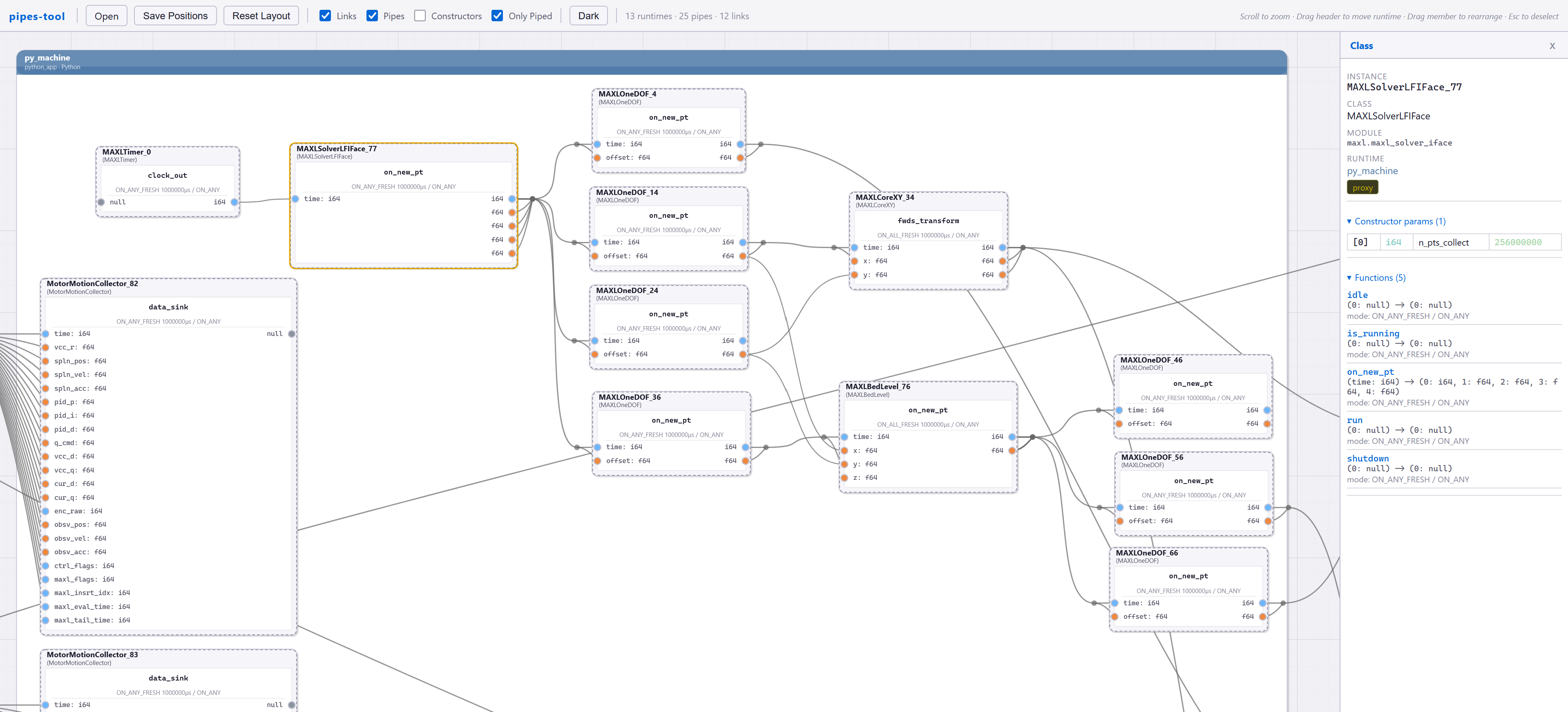
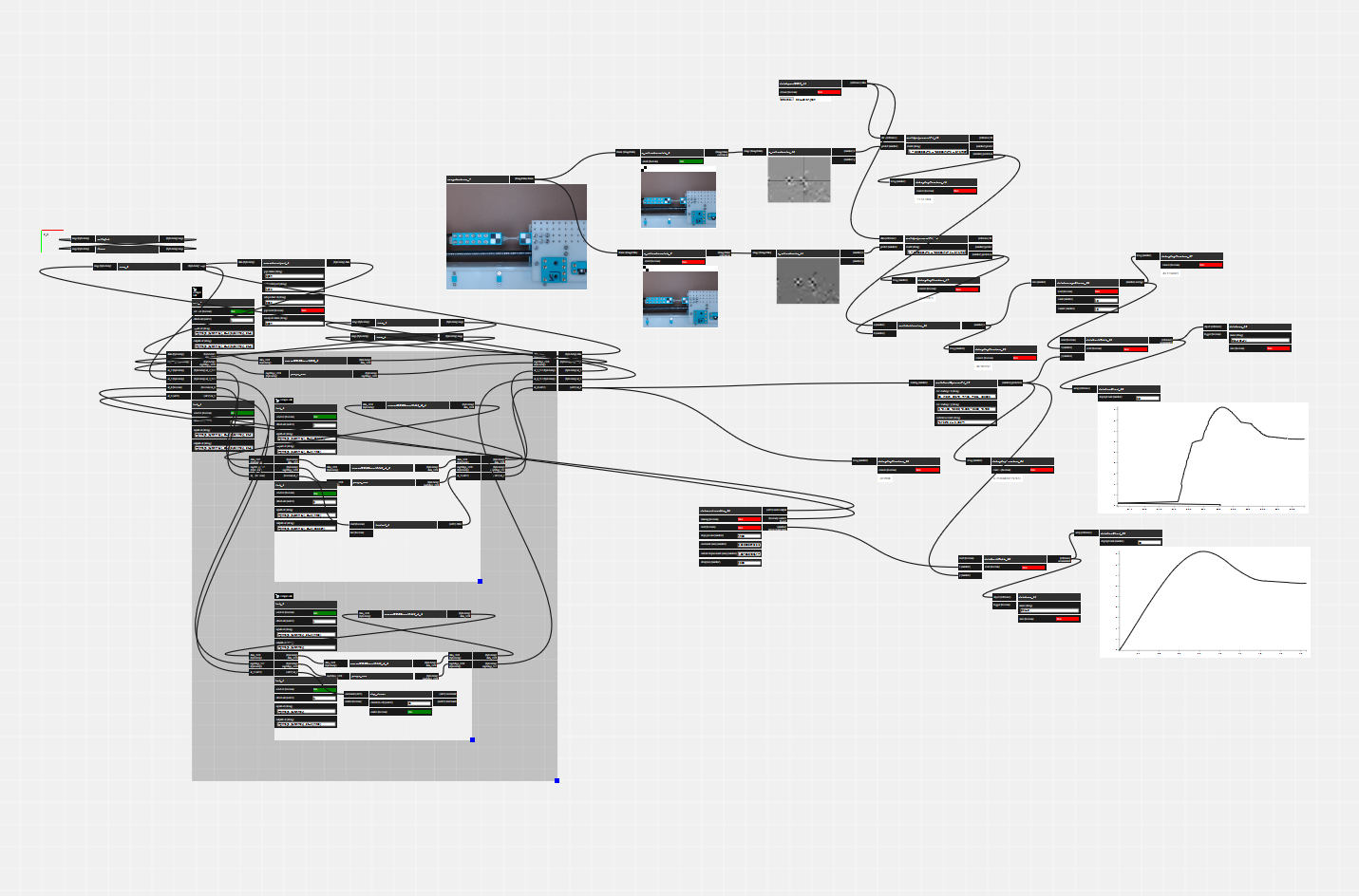
From Figure 1.9 and other discussion, it is clear that the systems deployed in this thesis are (1) always distributed and (2) sometimes messy. Structurally, they are all graphs, but I do not have a tool to visualize them as such. I would like to build a tool to do so.
A graph visualizer and editor would let systems developers quickly debug which hardware modules are connected, inspect their APIs, and build low-level data streams between devices. I have built a similar system in the past, but made the mistake of over burdening the graph representation: programs there had to be described entirely as graph entities. In an updated version, I would like to be able to interchangeably use scripting and graphs. I suspect that graph representations will be useful for low-level configurations, but that high level orchestration will take place using scripts.
(done) I plan also to include all of the graph editing API as script elements, meaning that a machine will be able to configure its own low-level systems; I anticipate that this may be useful for machines that need to alter their configurations during runtime, such as tool-changing systems.
3.6.5 Future Work for MAXL
3.6.5.1 Using Local Lookahead
For a final note, queuing motion as a function of time also opens up the possibility of using smaller lookahead controller within each device. As we drive performance of our motor drivers in the future (and continue to develop better models of these systems, and more embedded compute performance), using small Model Predictive Controllers for lookahead may become more prevalent and common (at the moment most practical controllers are simple PID loops). These require that each device has a future window of control commands to inspect, and time-encoded basis splines will be a useful representation in these cases.
In even simpler scenarios, some devices have known (and constant) lag times between actuation and output: for example an electromagnet or solenoid driven at the same voltage will always have the same delay (between when voltage is applied and when the target current is reached). Devices with fixed lag can simply inspect their target trajectory that many milliseconds in the future, and begin actuation ahead of time in order to delete lags.
3.6.5.2 Planning in Firmware
- Velocity planners are all authored in python/JAX, which is neat but troublesome at times for hardened machines. Especially for simple hardware that we just want to get up and running, and where we might want to use i.e. without dedicating a PC-scale computer to, we should be able to stick these planners in firmware.
- I mentioned in a few places the utility of moving velocity planners into software, only now to mention that we may want to move them back. However, I have also shown that a system like PIPES allows us to re-route controller dataflows: this could be used to easily inspect outputs from velocity planners in firmware, easily reconfiguring them as virtual controllers in the sense that they can be easily disconnected from their motors (etc) in test / inspection cases. This is known as hardware in the loop testing.
3.6.5.3 In-Firmware Safety Backstops
- Motion controllers developed by non-experts or in experimental schemes may generate erroneous outputs.
- Networks are never 100% reliable, and we will occasionally miss a packet. Recovering safely from these conditions is important. Spline interpolators in MAXL do have code to interpolate between lost points, if i.e. one in a neighbourhood is missing, but more robustness would prevent unsafe conditions when we have larger errors, like the complete failure of a network link.
- Using splines, motors can each run very simple maximum jerk, accel, velocity (position) computation: each incoming point is subject to this limit and if it lies outside of that point, we replace incoming point with the closes point within those bounds.
References
Networks tend to collapse when they approach their maximum utilization. The typical pattern is that increasing congestion starts to cause packet loss, after which transport layer algorithms begin queuing extra messages (retransmits), further increasing congestion. Once everyone starts doing this, links are quickly saturated and performance bottlenecks. Much work has gone into developing transport algorithms that intelligently avoid and recover from these scenarios, i.e. (that sick paper on networks as distributed optimization), and i.e. TCP New Vegas (which uses packet delay, rather than packet loss, as a flow-control signal).↩︎
Believe it or not, microwaves (like, for cooking your freezer dinner) emit radio waves near 2.4GHz (the same band as WiFi) at obscene power levels (1.5kW, whereas your laptop’s WiFi transciever will use about 100 milliWatts). If you run a network speed test and then reheat your coffee, you might notice that link speed degrading…↩︎
For an example from this thesis, the motor controllers (Section 5.4) are using all of their available 200MHz to servo the motors around. If we tried to stick the motion controller in there as well (and more motors), things would explode. This is additionally true for compute in general: datacenters and supercomputers rely on networks to expand compute volume beyond what is available on a single die.↩︎