8 Model-Based Control of a CNC Milling Machine
CNC Milling is at the heart of our manufacturing economy; milling machines are sometimes called “mother machines” as they are often the first stop when we make new machines (for any other process), molds, high performance prototypes, etc.
In this section I want to show that the tools and techniques I have developed thus far can be applied to this process, which is (like Chapter 7) constrained by real and measurable physics, but in practice relies on operators developing intuitions through messy abstractions - and lots of trial and error.
8.1 Direct Parameters vs. CNC Milling Phenomenology
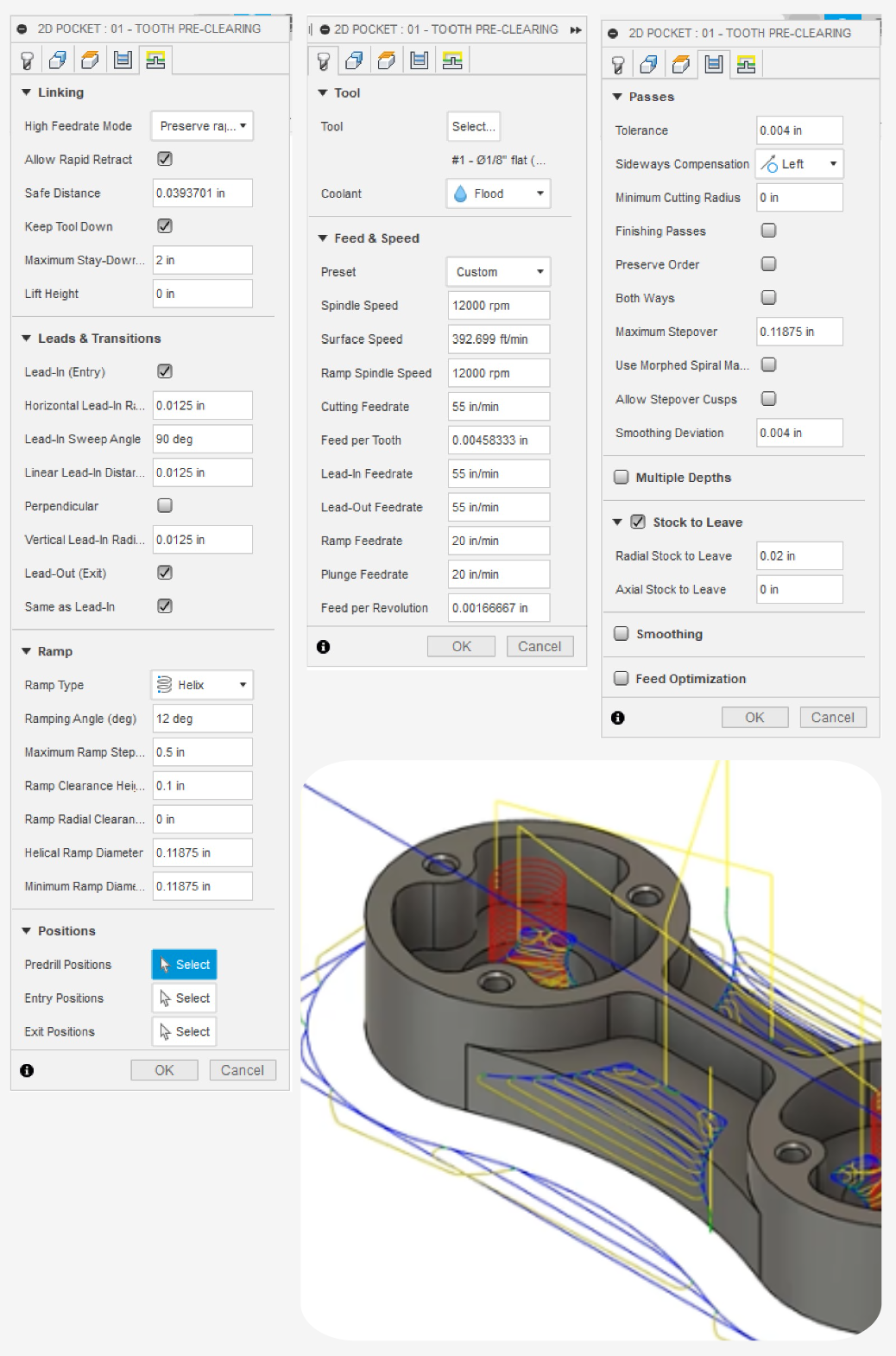
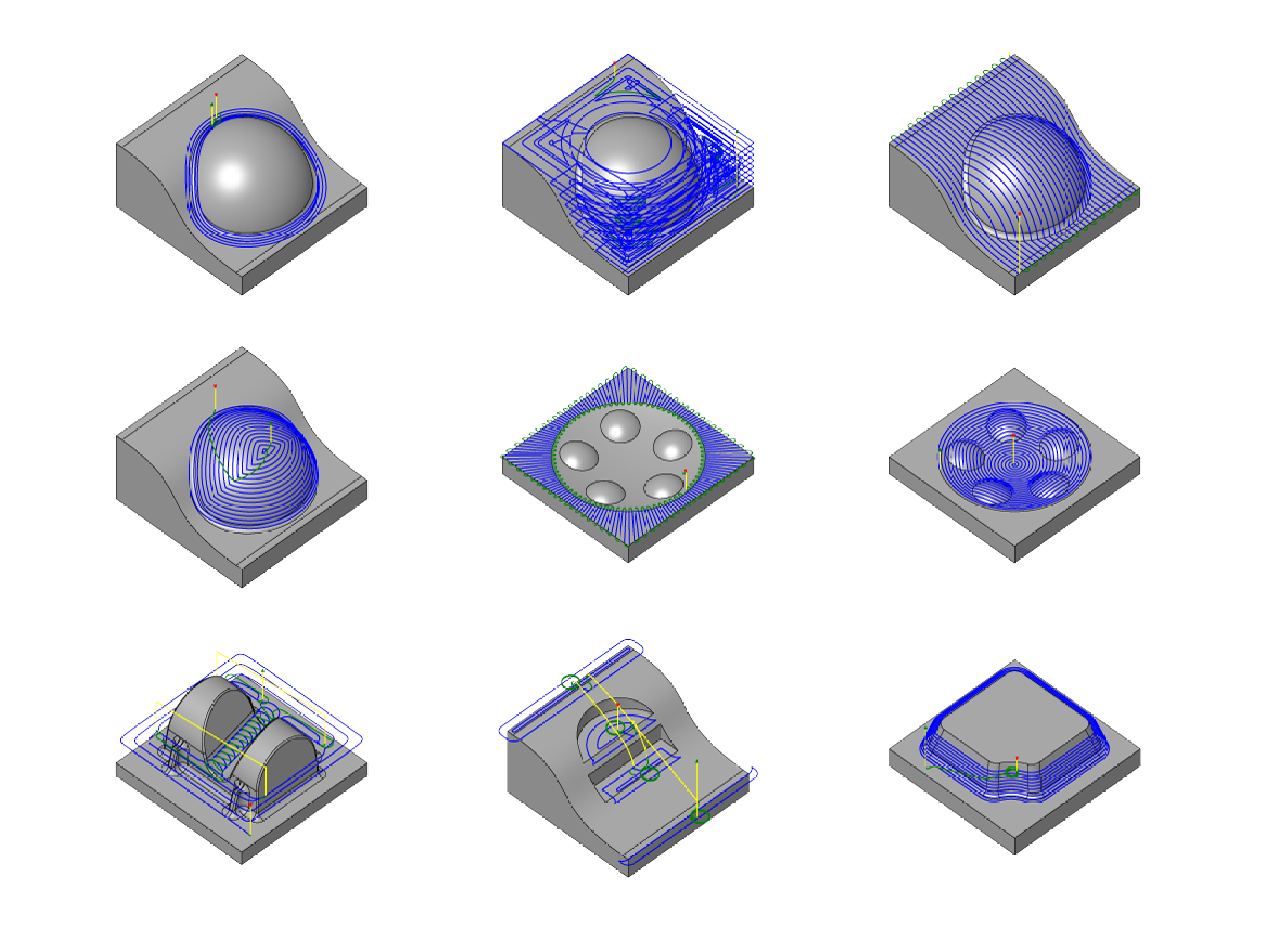
CAM for 3D Printing is at least simpler than CNC Machining because each job is one operation: slice into layers, produce perimeters and then infill for each layer. A machining job can include many (tens or hundreds) of different path planning strategies and tools for different geometric features, each selected manually. For example a tightly toleranced hole may require the machinist to select a purpose-made reamer, threaded features require threading tools, radiused or chamfered corners require fillet or chamfer end-mills, etc. I show a selection of these strategies in Figure 8.3.
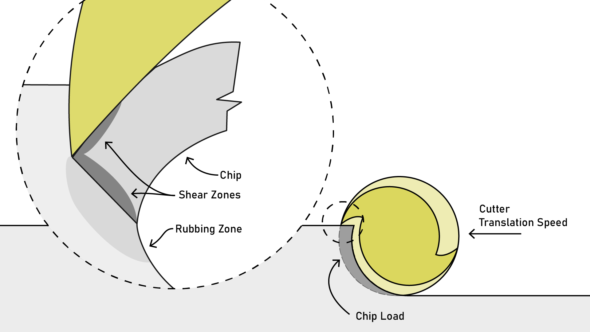
The physics of CNC milling is the physics of chip formation, which is mostly related to surface speed (how fast the cutter edge is moving with respect to the material), and chip load. These are both functions of the tool diameter, spindle RPM, as well as the machine’s linear traversal rate (which are the parameters we set in most CAM tools). Chip formation then generates overall loads on the machine’s structure that is related to the depth and width of the cut. Most complex of all in CNC Machining is the issue of resonance: any machine has a given natural frequency and if chip formation happens to excite the machine near that frequency, the whole system vibrates, causing innaccuracies or even tool breakage.
Milling parameters, then, are similar to FFF parameters: a user sets geometric and speed-related parameters that are only indirectly related to the underlying process physics that govern the system. Instead they are directly related to the low-level instructions (GCodes) that we send to the machine.
Essentially, the state of the art workflows have users writing low-level parameters directly, rather than describing high level goals or behaviours. This is akin to writing computer programs by directly authoring assembly language.
(previously in the intro) With CNC milling, deccelerating into a corner can change chip size dramatically, but because we cannot rapidly slow down spindle RPM (too much inertia!) we cannot simply scale the spindle RPM as a function of machine speed. Instead, we simply have a lossy layer: where we may setup a job to run at a particular chip size, some large proportion of the work might be done at much lower speeds with a much smaller chip size[^HSM].
8.2 An Instrumented CNC Machine
what is it, brother ? ratrig: stay simple ? try loadcell fit situation options or datron style, enclose-able but fer that pesky y axis ? leadscrews maybe preferrable to balls for the servo-loop settling damping ? perhaps it is most interesting to use i.e. a thick-ass belt drive machine for the milling, since its stiffness limits are tighter, to do more intelligent CAM: otherwise we are just competing SOTA vs. some half baked controller…
8.3 Modelling CNC Milling
8.3.1 Estimating Cutting Force
While the physics that generate cutting forces are intense (high shear rates, plastic deformation, heat and mass flow, etc…), we only need to model those physics if we want to look at cutting forces in small length scales: i.e. understand chip formation and evacuation, tool life, etc. In our case, we just want to understand the loads seen by the machine. A former CBA undergraduate researcher Chetan (who I was able to help out!) wrote his thesis on the topic (Sharma et al. 2021), I was also able to find another masters’ dissertation: (Dunwoody 2010). Both outline relatively simple models that output radial and tangential cutting forces as a function of straightforward geometric parameters (cutter size, cut depth, spindle rpm and linear feedrate), with four coefficients to fit for cutting force and edge force coefficients, each with tangential and radial coefficient respectively.
\[ \begin{aligned} F_t = K_{tc}ah(\theta) + K_{te}a \\ F_r = K_{rc}ah(\theta) + K_{re}a \\ \\ a = \text{cut area} \\ h = \text{cut height} \\ \theta = \text{chip thickness} \\ K_{tc}, K_{rc} = \text{cut force coefficients} \\ K_{te}, K_{re} = \text{edge force coefficients} \\ \end{aligned} \tag{8.1}\]
(Sharma et al. 2021) shows that coefficients can be estimated using data generated on-machine, using measured spindle power and force exerted on the workpiece (a loadcell). In this work, I essentially replicate Chetan’s measurement setup, building a CNC machine with loadcells installed between each axis’ ball nut and carriage, and I chat over RS-485 to the machine’s spindle controller to measure spindle load.
8.3.2 Pre-Processing Cutter Engagement
When we are fitting cutting forces, the most difficult task is measuring the engagement size. Chip thickness \(\theta\) is a simple function of our forwards velocity, flute count, and spindle RPM, but \(a, h\) are geometry dependent. To measure these, I develop a voxel-based preprocessor that steps toolpaths through the workpiece, using voxel intersections and removals to make a (quantized) chip engagement area per spatial step. Memory here is limiting, our voxel side length is 25 microns, filling up about 32GB of memory for a 100x100x50mm work piece.
8.3.3 Measuring Machine Stiffness
Adding loadcells to our milling machine is a wonderful tool, because we can measure the machine’s own stiffness. To do so, we clamp the spindle to the bed, and perform a test where we displace each axis while measuring load. Doing so, we can easily generate a stress strain curve for each axis.
8.3.4 Resonance Measurement
In this work, I only characterize and model cutting forces and machine stiffness (using those to optimize toolpaths to minimize deflection). I show that this lets us operate the machine in a deflection-limited manner, but in practice chatter causes more displacement than static loading. (Dunwoody 2010) adds resonance measurements: he uses a solenoid hammer to generate a step response of the tool, measuring the tools ‘ring’ using an inductive probe as a displacement sensor. Using this system, he generates a stability plot across spindle RPMs and depths of cut. In (Aslan and Altintas 2018), the authors develop a system that communicates with a Heidenhein machine controller at 10kHz to detect chatter in real-time using motor currents, and (Bort, Leonesio, and Bosetti 2016) develop a model-based adaptive controller to mitigate chatter and (Ward et al. 2021) implements a “machining digital twin” to optimize feedrates of a milling center in real-time to predict and automatically prevent chatter. Finally, for a broader overview of machining dynamics, we also have (Schmitz and Smith 2009) and (Altintaş and Budak 1995). I pass over this topic due to time (and, I should admit, skill issue) limitations, but show that our data contains enough information to characterize resonance.
8.4 Planning with Motion and Cutting Models
With the 3D Printer, I showed that we can build a controller that operates the hardware while respecting physical limits from machine motion, and the process. In this case we replace our flow models with a deflection model, and heuristics for i.e. layer height and cooling with model-based heuristics for cut geometry. This application is more limited than my work in 3D Printing (where I tried to develop an end-to-end workflow): here, I want only to show that we can model cutting forces using an instrumented machine, and use these forces to operate the machine under some maximum deflection.
The workflow here comprises a few steps, each a subsection here.
8.4.1 Building a Cutting Force Model for the Material and Tool
Like the 3D Printer, we need first to do some model fitting for each new material and tool. This is more cumbersome with machining because there are a wide variety of tools used in practice, each with new geometry, whereas in 3D printing we are basically choosing nozzle diameters alone. However, we can do similar open loop tests.
In this case I generate a test path that takes glancing passes at a square workpiece. The passes run at a series of cut depths (from 1/10th of the tool diameter to 2x the tool diameter), in increasing cut widths (from 1/20th of the tool diameter up to 1/2). When cuts exceed a pre-determined cut force, we stop incrementing the cut width (so that our test does not break the hardware).
FIGURE: img of test setup, + time series data collected
Using time-series data from these tests, aligned with pre-computed cutter engagement areas, we can fit the four parameters from Equation 8.1. We store these data for later use.
The tool’s own strength is also important: it is normally the case that the first physical limit a machine exceeds is to break the tool. In this work, I use simple beam models of tool geometry (with a significant safety factor) to estimate cutting force that the tool can withstand. The safety factor is adjusted to suit the tool’s geometry, i.e. relatively solid tools (with few flutes) use a smaller safety factor than intricate tools. A good piece of future work would involve using the machine to estimate tool stiffness, which could be done using a slew of methods available in the literature.
8.4.2 Using a Preprocessor for Toolpath Generation
In Section 7.4, I used a small pre-processor to pick high level parameters before handing jobs over to the realtime controller. I do the same thing here, but because this preprocessor modifes toolpath geometry, we have to do some manual steps.
I have greatly de-scoped this problem to manage only roughing passes in a machining geometry. In this regime our goals are simple: we want to remove as much material as possible without breaking the machine or tool.
In the first step, we want to select the variables that we cannot adjust quickly in our realtime controller: cut depth and width, and spindle speed. To extract these, we use some heuristics: we know that chip sizes should have some minimum - chips that are smaller than the tool’s edge radius get us into a scraping (not cutting) regime that quickly deletes tools. This gives us a limit to spindle RPM as a function of translation rate. We also know that it is better to move quickly through material taking relatively small passes, a true heuristic. To encode this, we set a minimum traversal rate. Finally, because we know that a high dynamic range of speeds can cause issues where our realized toolpath will vary from our target parameters (see Section 1.4.1), we set a maximum traversal rate such that our dynamic range between 90’ corners and wide open passes does not exceed \(100mm/s\). This generates for us a target cut width and depth, which we use to generate a toolpath using off-the-shelf CAM software.
FIGURE: Cut Area Calculator
Our realtime controller then needs cut area information. These data are not available in most CAM softwares, besides those that can be licensed at exorbitant costs. To supplement, I built a voxel-based tool that ingests a toolpath and stock geometry, segments the toolpath at a fixed spatial interval, and steps our tool through the part while removing voxels. The volume of voxels removed at each linear step defines our cut area. This signal is quantized and noisy, so we filter it slightly using a low pass filter whose bandwidth is just lower than the step size.
These generated codes are then serialized and saved to disk, where they can be picked up by our realtime controller for the next component.
8.4.3 Runtime Velocity Optimization for CNC Machining
With our processed toolpath, we can move to the runtime velocity optimization. This controller selects velocities along the toolpath such that the machine’s actuator limits are not violated, using motor models, inertial and kinematic models, and a cutting force model.
FIGURE: the velocity controller: motor, spindle loads…
In the state of the art, velocity controllers don’t have (or use) information about cut geometry. However, motion dynamics change drastically when a machine enters and exits a cut: torque bandwidth during a cut is more limited due to the amperage required to maintain cutting force, whereas in a jog (or ‘rapid’) move, we have the full actuator requirements available.
The velocity controller uses a few items in the cost function. As is the case across machines, it calculates motor currents at each step and selects velocities that prevent these currents from exceeding their maximum. It does so as well for \(di/dt\), which is limited by motor inductances. Recall that currents also reflect cutting forces from the model. In this machine, we add a deflection criteria, i.e. minimize total dynamic loads (from inertia and cutting forces) so that the kinematic chain’s precision is maintained during operation.
8.5 Comparison of Simulated Toolpaths with Time-Series Data
Here I will show results from machining operations: comparing simulated loads and motor currents to measurements from the machine.
8.6 Learning from Milling Machine Models
As I showed in Section 7.6.3, we can learn from our machining operations. The machining model is oddly simpler than that of FFF printing, but mostly because I have left out the meatiest factor, which is chatter. Here we can see that we can essentially bin toolpath segments into three categories: moments where we are limited by the machine’s inertia (in corners and detailed zones), moments where we are limited by the actuator’s ability to produce a cutting force, and moments where we are limited by the machine’s stiffness.