6 Motion Control using Machine Models
In the previous chapter I explained how I stream motion signals to motors and actuators, now we will look at how we can optimally generate those signals to move the machine as quickly as possible without exceeding our actuators’ limits.
Motion control is an apparently simple task that turns out to be more nuanced than many anticipate. In fact it is a full blown constrained optimization problem - this can be intimidating for folks who haven’t eaten their maths vegetables1. In this chapter, I hope to explain it in a manner that is approachable to folks who have (say) done lots of mechanical design and want to understand (or build) the algorithsm that make their machines graceful and performant. I will assume that the reader has a basic background in programming, mechanism design, and some controls (i.e. PID). Even just a curiousity with any of those topics should suffice.
Motion control expands to generalized trajectory optimization (Tedrake 2024b) (which includes choosing path geometries as well as velocities) but in this case we are going to focus on a simpler subset: velocity optimization along a given path. This formulation is often called “acceleration control” or “acceleration planning” - depends on who you are talking to. It is also called “lookahead planning” because it requires that we look forwards towards the next corners in our trajectory in order to figure out when we need to start stopping (i.e. pick a breaking point) so that we don’t end up going too fast at the corner in order to make it through the corner precisely.
In this work I am developing a model based motion controller, meaning we are going to use mathematic representations of our system’s actuators and dynamics to optimize against. So, I will take us first through a review on electric motor physics (and a section on the motor controller that I developed and use), then look at models for motion of mechanisms (kinematics, inertias and damping), and briefly at machine resonance modeling and its relationship to stiffness. I will also review common motion control formulations like trapezoid / s-curve generation and junction deviation and explain how they relate heuristically to those physical models.
Finally, I will explain the motion planner that I have developed, which is framed more directly as an optimization problem (rather than as a set of heuristics + dynamic programming (Tedrake 2024a)). I will compare trajectories generated in this solver to those generated by heuristics based planners, and show how the model based planner out performs heuristics. In the next chapter, I will show how optimization based planners can be extended to include process dynamics alongside motion dynamics.
6.1 Motor Control and Modelling
Motor physics are the most foundational for motion planning: as discussed, we need to understand these physics to know what our constraints are going to look like. This means electric motors: probably motion control is possible with turbines or internal combustion (and certainly it is possible with hydraulics and pneumatics2), but I am not going to get into it for the reasons you can probably imagine.
In this section, I will first introduce the hardware and core control algorithms I used for motor control, and then discuss how I used that motor driver to build motor models that we can use in the motion controller.
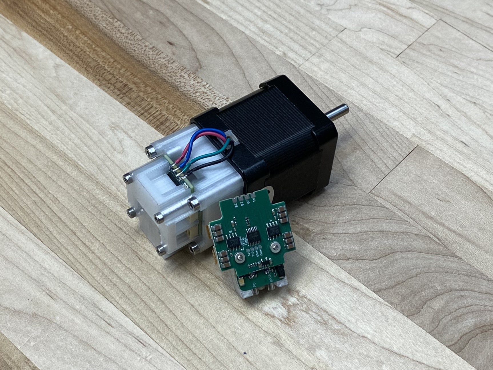
6.1.1 FOC on (almost) Any Stepper
- steppers ubiquitous and available in a heterogeneity of form factors at low cost,
- controls are typically lacking closed-loop and model discovery, but we can drive them like servos, gaining both back,
- the controller hardware, firmware,
- model discovery: L, R, encoder calibration (and DQ variable L ?) -> kt==ke, k_controller (and encoder noise),
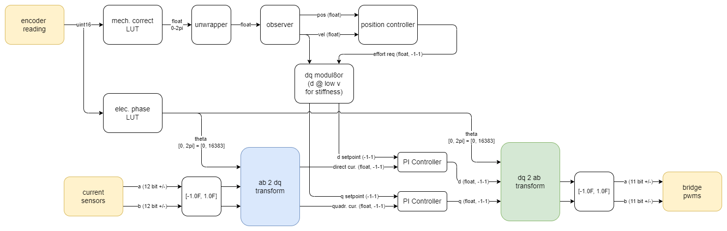
- PWM and current sampling / sign discrimination, PI controllers, DQ/AB transforms,
- kalman observer (and tuning ?)
- PID spline following
6.1.2 Modelling Motors
To start, let’s look at the classic electric motor and model:
Stator, Rotor, Fields, Etc
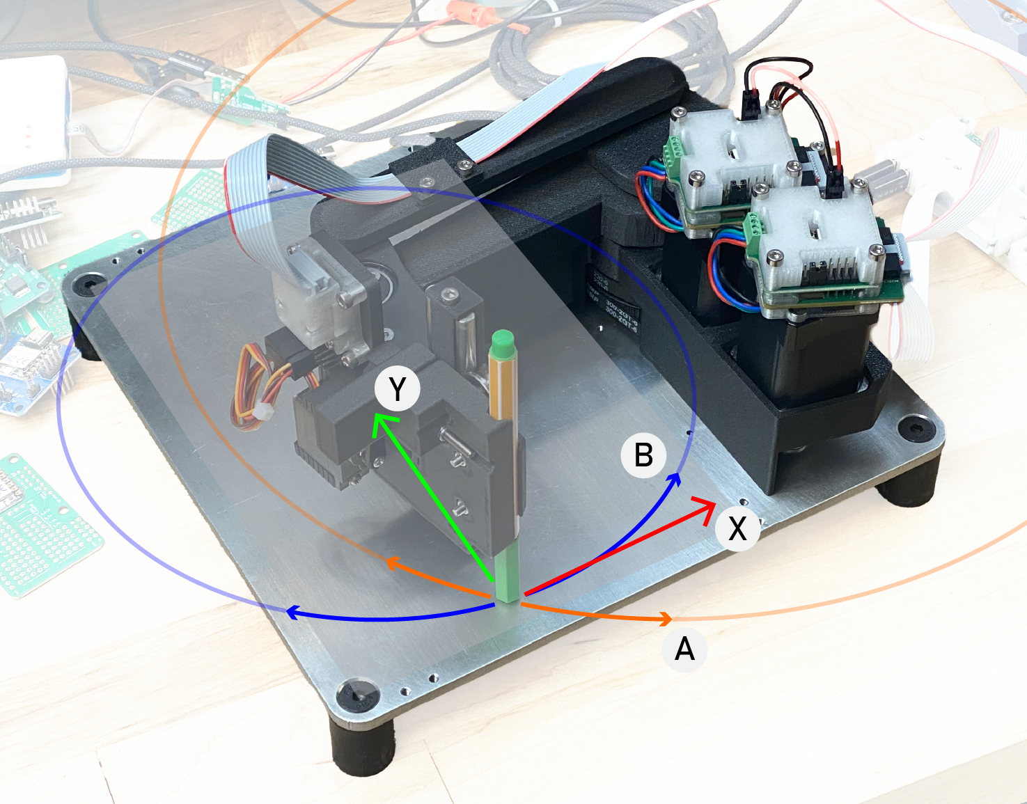
Our motor has a stator (the static part) with electromagnetic windings that can generate a magnetic field, and a rotor that has a permanent magnetic field. Because I use them in this work, I have drawn the electrical diagram of a stepper motor, which has two independent stator windings A and B. Many other motor architectures exist, but the concept (and modelling) is fairly consistent across each.
When the motor is operating, we switch current in the stator to motivate the rotor to rotate. For example when we drive positive current in A and zero current in B, the stator’s magnetic field points “up” and the rotor will move to align with this current. When the stator field is 90’ out of alignment with the rotor’s field we produce maximum torque, and during operation we continually update the stator’s magnetic field in order to maintain this relationship (a process called commutation).
The motor physics breaks down in to three constitutive equations:
\[V = RI + L\dot{I}\] \[\dot{I} = \frac{V - RI}{L} (?)\] \[I = \frac{V_a - k_e\dot{\Theta}}{Z}\] \[Z = \sqrt{R^2 + \dot{\Theta} L^2}\] ^ right ? - and maybe we should use \(\omega\) for speed, as is more common ?
\[Q = k_tI\] \[\ddot{\Theta}J = Q - k_d\dot{\Theta}\]
| Parameter (units) | Name | Meaning |
|---|---|---|
| \(V_a\) \((Volts)\) | Applied Voltage | Voltage applied by the driver to the stator coils |
| \(V\) \((Volts)\) | Stator Voltage | Voltage in the stator coils |
| \(A\) \((Amps)\) | Stator Amperage | Current in the stator coils |
| \(R\) \((Ohms)\) | Stator Resistance | Windings’ DC Resistance |
| \(L\) \((Henries)\) | Stator Inductance | Windings’ Inductance |
| \(Q\) \((Nm)\) | Torque | |
| \(J\) \((kg \cdot m^2)\) | Rotor Inertia | |
| \(\Theta\) \((radians)\) | Rotor Angle | |
| \(\dot{\Theta}\) \((radians/s)\) | Rotor Velocity | |
| \(\ddot{\Theta}\) \((radians/s^2)\) | Rotor Acceleration | |
| \(k_d\) \((Nm/rad/s)\) | Damping Factor | Friction! |
| \(k_t\) \((Nm/Amp)\) | Torque Constant | How much torque is produced per Amp of current in the stator. |
| \(k_e\) \((Volts/rad/s)\) | Back-EMF Constant | Voltage induced in the stator by the rotor’s magnetic field. |
Most of these values can be easily measured in the real world: \(R\) is a simple multimeter test, and \(L\) can be measured using an LCR probe. \(V\) and \(A\) are measured in the motor controller’s firmware, \(\Theta\) (and its derivatives for velocity, acceleration) are also measured in firmware (using an encoder). Rotor Inertia \(J\) is typically included in a motor datasheet, but I have at times taken motors apart to weigh and measure this when datasheets seem untrustworthy. That leaves \(k_t\) and \(k_d\) to fit computationally, which we will see later (alongside easier ways to estimate some of the other parameters). To arrive at these values computationally, we would need complex simulations of the motor’s internal structure: winding counts, magnetic properties of stator and rotor steel and permanent magnets, etc - this is not worth it, so we fit to data instead.
A few things are worth noting about the motor model. Firstly, by the magic of SI units, \(k_t\) and \(k_e\) are equivalent (although they have different physical meanings). One way to intuit this is that they both describe the interaction between the rotor and stator’s magnetic fields: \(k_t\) tells us ~ how much the stator’s field pulls on the rotor’s field, and \(k_e\) tells us ~ how much the rotor’s field drives voltage in the stator’s windings. If you squint the third eye, this can make a lot of sense. For a better explainer, I will paraphrase a fantastic stack overflow post (REF: we will have to go digging thru the motor control notes for that)
TODO: paraphrased explainer from above…
Second, we see that torque generation is based on stator currents, and that stator currents are limited by a few factors. Out of band from the model itself are the saturation limits of our controller hardware: we do not have infinite voltage available, and there is a limit to how much current our switching electronics can source before they explode. These limit the current that we can drive when the motor is at a standstill.
Once the motor gets going, our voltage is quickly reduced by Back EMF. BEMF is the voltage generated by the rotor’s magnetic field spinning inside of the stator’s coils: i.e. recall that any electric motor is also a generator. As the motor nears its top speed, the voltage generated by the spinning rotor is almost equivalent to the voltage applied by the controller, and so the effective voltage across the stator’s windings goes towards zero.
In another limit to top speed, the stator coils impedance increases as a function of the rotor speed. Impedance of any electrical component is essentially AC resistance: it is measured in ohms and describes how much the component resists (or… impedes) current flow. This has an additional speed-scaling effect: as we commutate the stator current at an increasing frequency, we need even more voltage to drive the same current into the stator.
Finally, we see that the current in the stator (and so the torque) is impossible to change instantaneously… \(\dot{I} = ...\) - this is why we want to have jerk limited trajectories: instantaneous changes to acceleration require instantaneous changes to current, which our machines cannot realistically achieve. We will look in more detail later (SECTION?) at how these properties can be used to heuristically estimate maximum possible jerk for a given system.
Sometimes it is easier to understand models if we look instead at the code that simulates them, so I am including here also a snippet of python code that runs this model and plots the system outputs.
LISTING: motor model example code (including saturations)
Motor w/ Big Rotor-Dyno
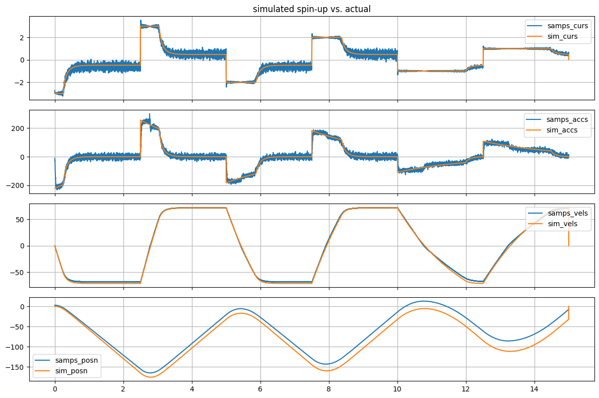
In the code snippet (and output simulation), we can see the effects discussed at work: at low speeds, current driver saturation is our primary limit, but when speed increases we see a two-fold (quadratic looking) dropoff in the available current and torque. Finally, as speed of the rotor increases we see more physical damping take place, further limiting our top speed.
Using this simulation, we can generate a plot of the maximum positive torque available from the motor across a range of speeds.
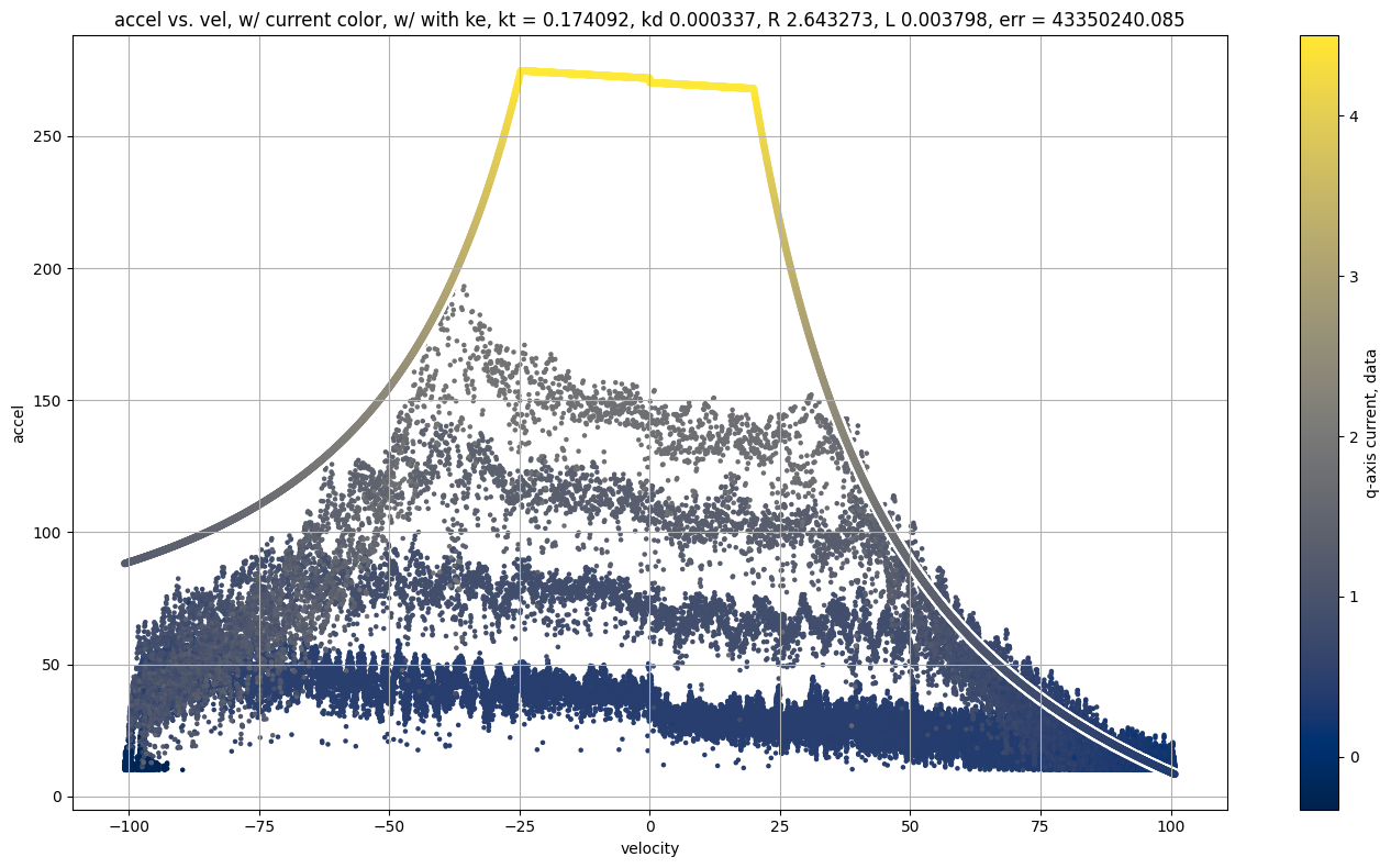
The torque curve is an excellent tool and they are commonly used by machine designers to select actuators, for example if we know that an axis of our machine will mostly be responsible for fast accelerations at low speeds, we will pick a motor with more torque “in the low end,” whereas if we have a large gear ratio and need our motor to work at large RPMs, we will look for motors where the torque does not fall off drastically as speed increases. Later on, we will also see how torque curves can be used to heuristically select maximum accelerations, velocities, and jerks.
6.2 Kinematics and Inertias
Except in some rare cases, motors don’t drive machine components directly. They are connected via belt drives, leadscrews and ballscrews, gearboxes (etc) or combinations of each. Understanding the machine’s kinematics enables us to translate between the machine motion we are interested in controlling, and the motor models (and stiffnesses) that constrain that motion.
For the purposes of the current topic, it is sufficient to model the machine as a set of rigid bodies, and deal with stiffness only in the frequency domain. We will also only cover kinematic systems where any set of actuator positions corresponds to only one possible machine position, and vice/versa.
this block came from the proposal intro !
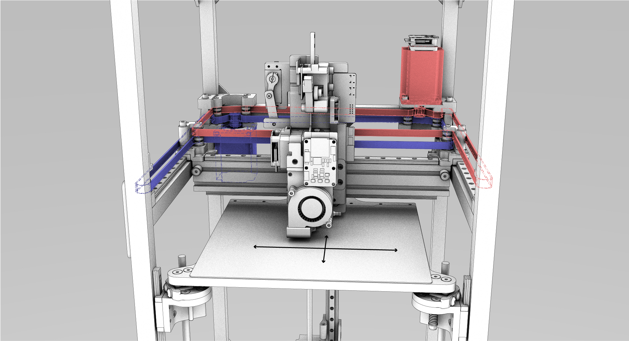
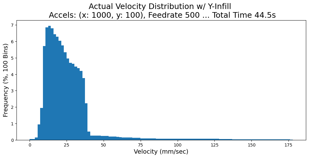
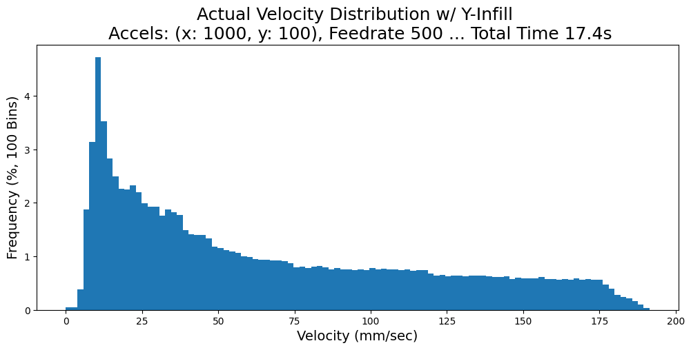
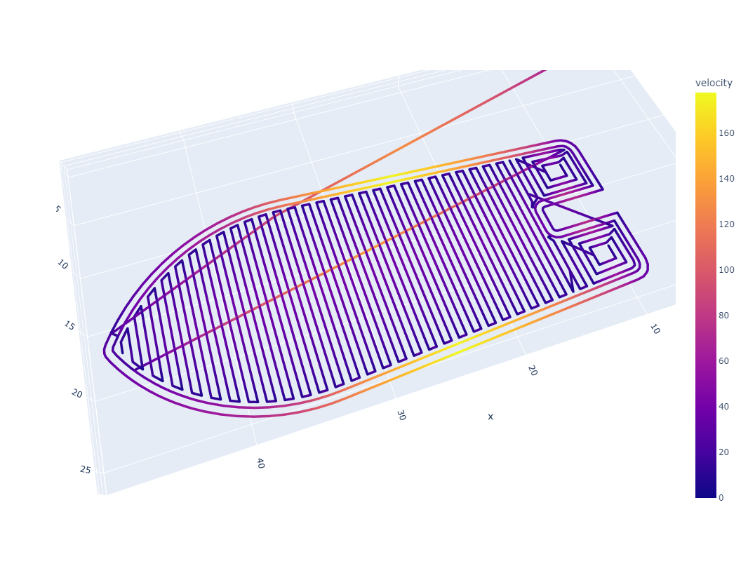
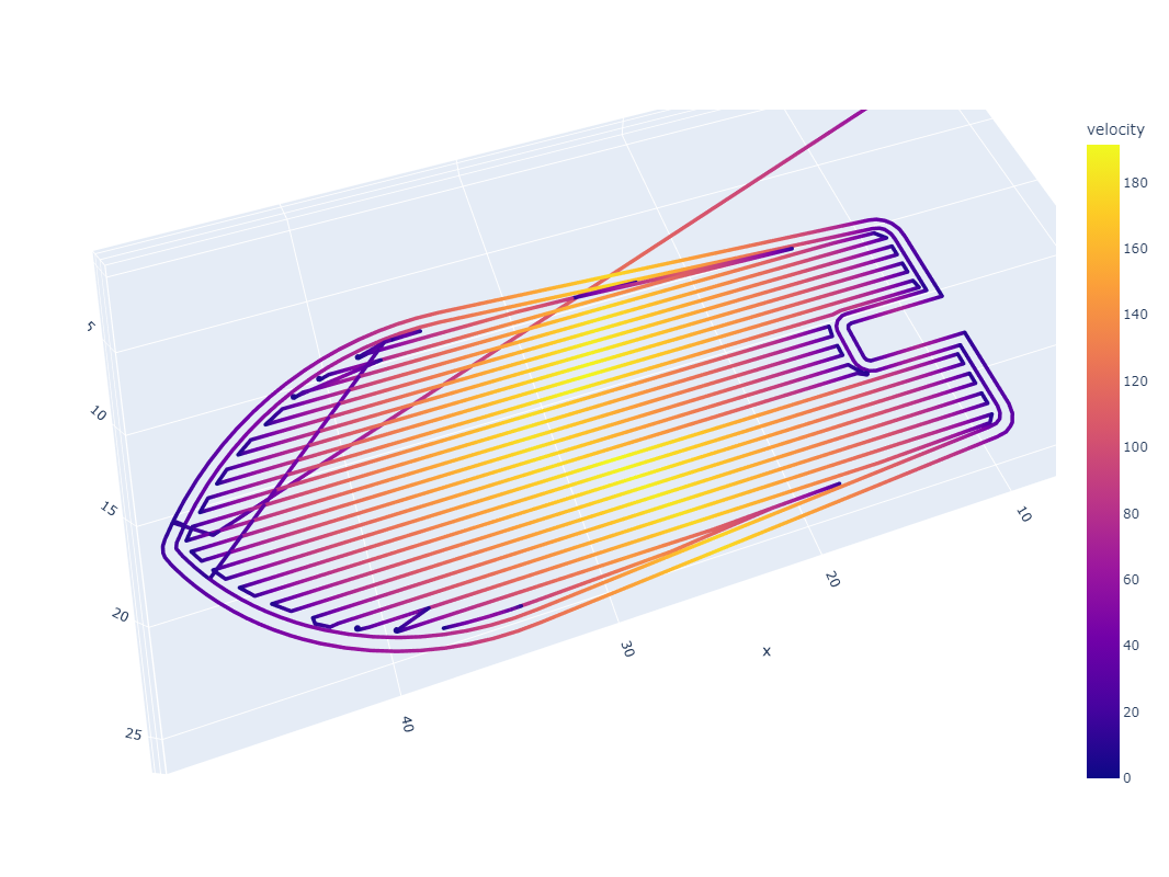
Switching directions quickly is important for any machine, and machine builders have developed novel kinematics to increase performance in this regard. One of which is CoreXY (Moyer 2024). CoreXY (and many other arrangements) is anisotropic in its physical speed and acceleration limits: it has to move much less mass in the X direction than in Y - while it has just as much available motive force in either direction. This means that a part’s orientation with respect to the machine’s kinematics can be hugely important for overall print speed, as shown below in Figure 6.6. Slicers, however, are unaware of this property, meaning that they can’t optimize print speeds by (for example) changing the primary direction of an infill pattern.
| With Infill Misaligned to Anisotropic Acceleration Limits | With Infill Aligned to Anisotropic Acceleration Limits |
|---|---|
 |
 |
 |
 |
CoreXY
Bell Everman Kaos Kinematics
Scara Kinematics
- Kinematics, Actuators, Inertias
- that middle step: we need transforms between actuators (and their models, inertias), and outputs… the planner needs this in order to transform v(s) into actuator currents, etc
- nonlinear vs. linear transforms… and singularities ?
- each transform describes how a position (actuators) is transformed into a position (wcs), or vice-versa, and those derivatives are (?) jacobians…
6.3 Stiffness and Resonance
- Mechanical Resonance
- everything vibrates… exciting resonances is bad,
- using an acceleromter, we can send input
chirpthru motion system in each mechanical DOF, and FFT the output to find peaks… - difference between measured acceleration and end effector and measured at motors, thru kinematic model, is related to stiffness of system,
- current @ motors, thru model, relates to damping,
Freq. Response of CoreXY
V/T w/o Resonance Delete
V/T w/ Resonance Delete
6.4 Velocity Planning
Introduce problem / topic; is Section 1.4.1 related: we must constrain velocities to respect system limits.
Advances in differentiable simulation and solvers have made it possible to refactor machine controllers as online optimization routines, but it is still unclear how to put all of the constituent pieces together.
The proposed optimizer also has clear performance metrics to measure: it should help machines run closer to their maximum limits, minimizing time to run jobs and maximizing precision.
6.4.1 Common Approaches to Velocity Planning
is s-curve / trapezoid generation, accel, jerk limits, (point out the… square area under the curve), junction deviation, or (better) arc insertion, tying processes in to these planners can be cumbersome, as they use incomplete models and “think linearly” - i.e. we can’t arbitrarily add constraints - the soln’ presented here is flexible in that we can basically throw whatever tf we want into the solvers’ cost function, and we lean on GPU / AutoDiff magic to make it work… this comes at the downside of being less deterministic, und-so local correction and control (?) in many such systems, we simply pick maximum velocity, acceleration, and (sometimes) jerk - rather than working from models of motors and kinematics in order to pick those optimally. the formulations also prevent us from using the full dynamic range, as we have (?) already explained
6.4.2 Background in Constrained Optimization and Differentiable Simulation
State of the art machine workflows are implicit constrained optimization problems: users want to make their parts precisely and quickly, but they are limited by process physics, material properties, and machine dynamics. As I’ve explained, this optimization is currently distributed across two disconnected systems (CAM and the Controller), and is articulated somewhat awkwardly with indirect parameters leading to difficult-to-discern differences in outcome. The optimization is not made explicit anywhere, nor are the physics written down anywhere - people rely on heuristics above all and the whole process is feed forward: we tune systems until they break.
In this thesis I propose to replace big parts of these workflows with models and numerical optimization, and bring them together into accessible, interpretable programs. I am enabled to do this largely because of new availability of autograd tools, that automatically generate gradients for any given program (a key ingredient for optimization). In particular, I am using JAX (Research 2024). With JAX, any system that can be articulated as a purely functional python code can be automatically differentiated. We can then use the function’s gradient to optimize the function’s inputs, and JAX conveniently pairs with optimizers from the OPTAX library (DeepMind 2024). The performance of this system is only viable because JAX also includes a just-in-time compiler that turns the whole system into code that can run in parallel on high performance hardware (i.e. a GPU).
MAXL uses JAX as a basis to implement a Model Predictive Controller (Brunton and Kutz 2022a). MPC controllers work in much the same way as you and I do: it uses a simulation of the future to optimize future and current control outputs. The classic example comes from driving: when we are entering a corner, we know that we need to slow down before we turn. To pick a braking point, we use a mental model of our car’s dynamics (how long it takes to slow down) to “simulate” (imagine) how long it will take to come to the appropriate entry speed for the corner. With computational MPC, we simulate and optimize control outputs over a horizon of up to a few seconds at each time step, but only issue the immediate next control output to our system. For example in the solver that I have implemented, I optimize 250ms of control outputs at a 4ms interval, every 4ms. MPC is slightly more complex than other common controllers because it involves building system models, but its flexibility makes it well suited to many tasks, probably the most popular of which is in robot quadrupeds (Di Carlo et al. 2018) quadrotors (Torrente et al. 2021) and humanoid robots (Kuindersma et al. 2016).
Most MPC researchers use software libraries for these tasks: CasADi (Andersson et al. 2019) and ACADOS (Verschueren et al. 2021). CasADi lets developers author symbolic representations of their system dynamics and cost functions, the package then generates C code for evaluating derivatives and integrating dynamics models. ACADOS is a solver that can directly use those C codes to minimize cost functions in real-time. This follows a similar pattern to the one I am deploying with JAX, but in this case I am using JAX both to define the system (using pure python functions) and solve the system (using a JIT-compiled optimization step). The key difference is that the CasADi / ACADOS workflow targets execution on embedded devices. It is probably much more efficient, but harder to update with new models (requiring a more explicit compilation step).
MPCs are typically used for short-order optimizations, operating over time horizons around one to five seconds. They usually run somewhere between 50Hz and 500Hz since the compute required to solve them is intense. For longer horizons of control, the current best practice uses simulated systems to train policy controllers (Brunton and Kutz 2022b) that can issue higher-level control commands. Policy controllers are normally coupled with lower level, faster feedback controllers and classical controls components like kalman filters, (Kaufmann et al. 2023) is a particularely clear example of how all of these components come together to produce performant controllers. Policy controllers are often trained without gradients because it is hard to differentiate across long time spans, but recent work deploys differentiable simulation to overcome this issue (Song, Kim, and Scaramuzza 2024).
All told, optimization based control is a vast, complex discipline. I have not mastered any of it, but the available tools have become sophisticated enough that I can generate a solver using my own models and deploy it in practice. Above all, this is a testament to the community of researchers and engineers working together to advance the practice, who are committed to sharing reproduceable, useful tools with one another.
6.4.3 Optimization Based Motion Planning
it’s the JAX Section: how does planner work diagramatically, where models, where optimizer choices, where cost function ?
LISTING below is from the proposal, is broken: we want to show the motor model (those are above?) and the snippet from how the solver calculates motor currents given vi, vf @ some trajectory ?
def integrate_pos(torques, vel, pos, del_t):
    params_torques = jnp.array([2000, 1000])  # per-axis motor effort to torque
    params_frictional = jnp.array([2, 2])     # per-axis damping

    torques = jnp.clip(torques, -1, 1)
    torques = torques * params_torques

    acc = torques - params_frictional * vel
    vel = vel + acc * del_t
    pos = pos + vel * del_t

return acc, vel, pos- background: we need to lookahead so that our x(t) respects actuator constraints (models!)
- many SOA are accel or jerk-limited
s-curves- this basically represent using some “square” block of area under the torque curve of a motor, - in SOA, segments are linked w/ JD (sometimes)… literature on what the fancy folks @ siemens etc is limited (?)
- many SOA are accel or jerk-limited
- solving via optimization…
- yada yada, yada…
- where do models come from and where do they go ? (motor components, inertial / damping components, and motor transforms…)
- parallelizing the solve ?
- etc, etc,
- energy @ frequency deletion ?
- connecting the solver (big nasty process) with the machine architecture:
- solver is a block of code… timer in -> triggers new solutions, pipes time-parameterized chunks out to hardware
- time scales: we can solve at around or just under realtime, so we run these simultaneously, though we are not closing this loop at the high level: servos are doing that…
6.4.4 Deploying Model Based Motion Control
- workflow: motors models, inertia masses, -> chirp estimates stiffness, resonance, damping -> solutions…
- evaluation here: optimized plotters + what we learn from machines (motion component)
- compare to square-area-under-torque-curve solvers,
- whereis trajectory limited by which… motor, inertia, damping term ?
- can we relate FFT force:resonance to springrates, damping rates, and learn this about our machines ?
- plotters-comp ?
My initial attempts used a direct shooting representation(CITE: Tedrake), where the optimizer’s decision variables3 are the control variables that we use to simulate the output. These are i.e. the currents that will be used by the actuators at each step in the simulation. In direct shooting, we start from an initial set of states (positions, velocities), and then apply the first set of u_{t0} (explain…) to the system, to generate the next time step’s output. From those states, we then take the next u_{t+1} and integrate again, and so on. Direct shooting has the property that it is guaranteed to produce outputs that are feasible (if our u are appropriately scaled), but it has the result that all computations are sequential: i.e. we need the states from t to generate the initial states for t+1. This is undesireable because it cannot be parallelized on modern compute hardware.
… the well known alternative is direct transcription(Tedrake again), where we use as decision variables all of the states of the system, as well as the control inputs. We can then parallelize the computation, given that at the outset we have all x(t) and can predict all x(t+1) in parallel. Because this breaks the time dependence that guarantees our global trajectory will “link up” (i.e. x(t) -> x(t+1) match the model), we need to have the solver also implicitly solve for this linking. Coming from the world of simulation, this seems like an insane solution, but the gain we get from parallelizing the system is huge if we have the available compute hardware. It also has the effect that the derivatives of the solution are not chained together… (? more on that?).
I implemented a direct transcription solver as well, but was unable to have it converge cleanly for given trajectories. Mostly I struggled to have it turn corners (believe it or not), since it was able to find clean solutions where it simply stopped in front of a corner… yada yada.
The breakthrough for me came in articulating the solution in “phase space” - which is a fancy way of saying that the solver uses fixed increments along the spatial trajectory rather than fixed increments in time - this has the effect of causing any given corner to always remain in view of the solver, to force it to come up with a solution for the same. In introduces its own problems, which I will get into later.
… yada yada, yada, we’re going to have to actually write down a bunch of math in this one.
… “so you’re telling me I need a GPU to control my machine?”
I know, it seems insane. While this controller is measurably better than other solutions, it needs to run on some expensive computing hardware. For example, during the development of this thesis I used an RTX 4070 GPU ($700) to run machines whose BOM costs were between $200 and $800 each. Of course this trade-off might not seem as insane were we talking about half-million dollar milling machines.
Two notes on that: first, this is the advantage of being a researcher: we can occasionally make insanely strange economic choices and then simply make statement like (second note:) compute hardware for “AI” (i.e. GPUs) is currently one of the most over-invested fields in the world. At the time of writing, NVIDIA’s (who makes GPUs) valuation is something like 7% of the USA’s GDP. Smells like a bubble to me, but when this one pops the cost of this computing hardware will be a tenth of what it is currently.
A third note on that is that the optimizers developed here do not need big GPUs, just baby ones. This application takes up only 200Mb of VRAM, for example. The oracles in the (silicon) valley would expect the level of GPU required here is likely to be available for tens-of-dollars in the near future.
6.5 Learning from Model-Based Machine Control
6.5.1 S-Curves vs. Model-Based Control
FIGURE: per-machine, comparing outputs to show that our solver can generate faster trajectories, with less resonant excitation (accel histogram vs. planned accel histogram ?)
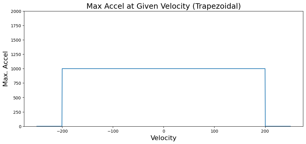
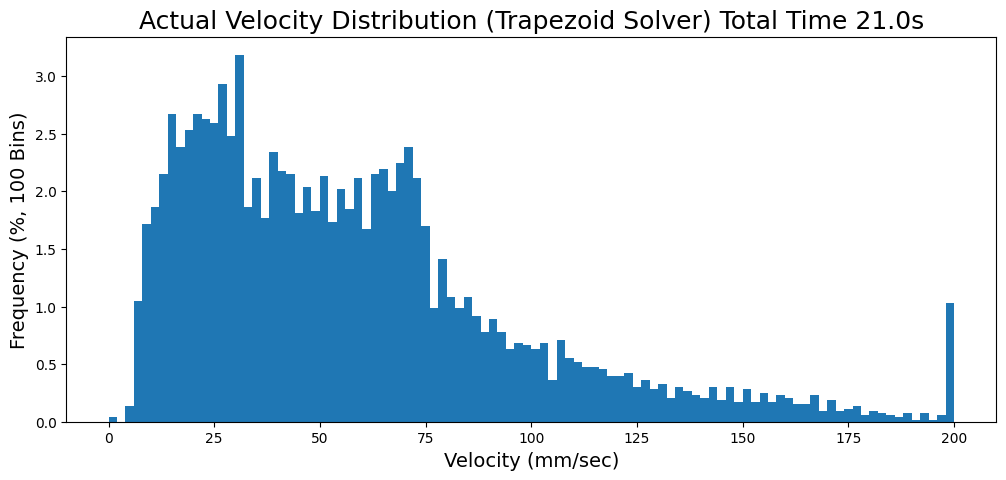
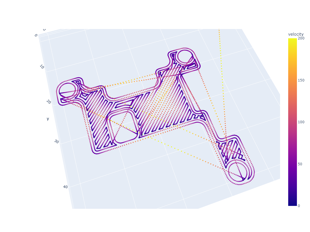
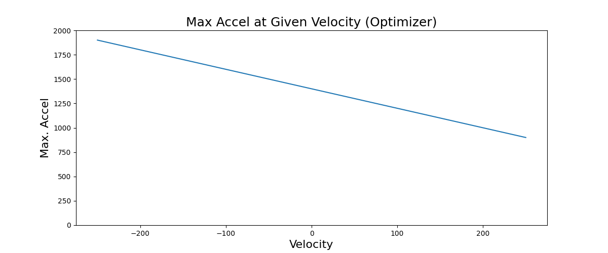
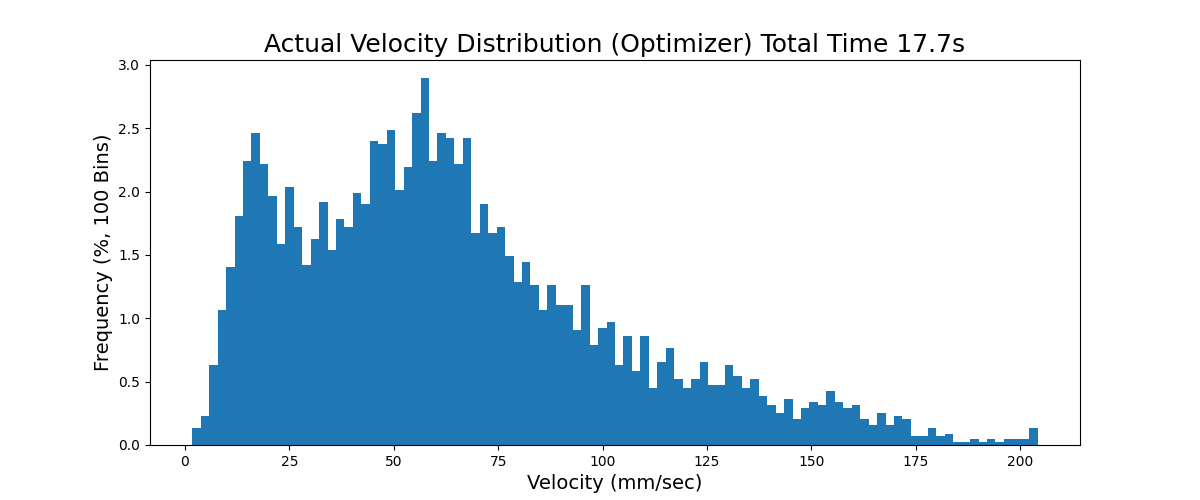
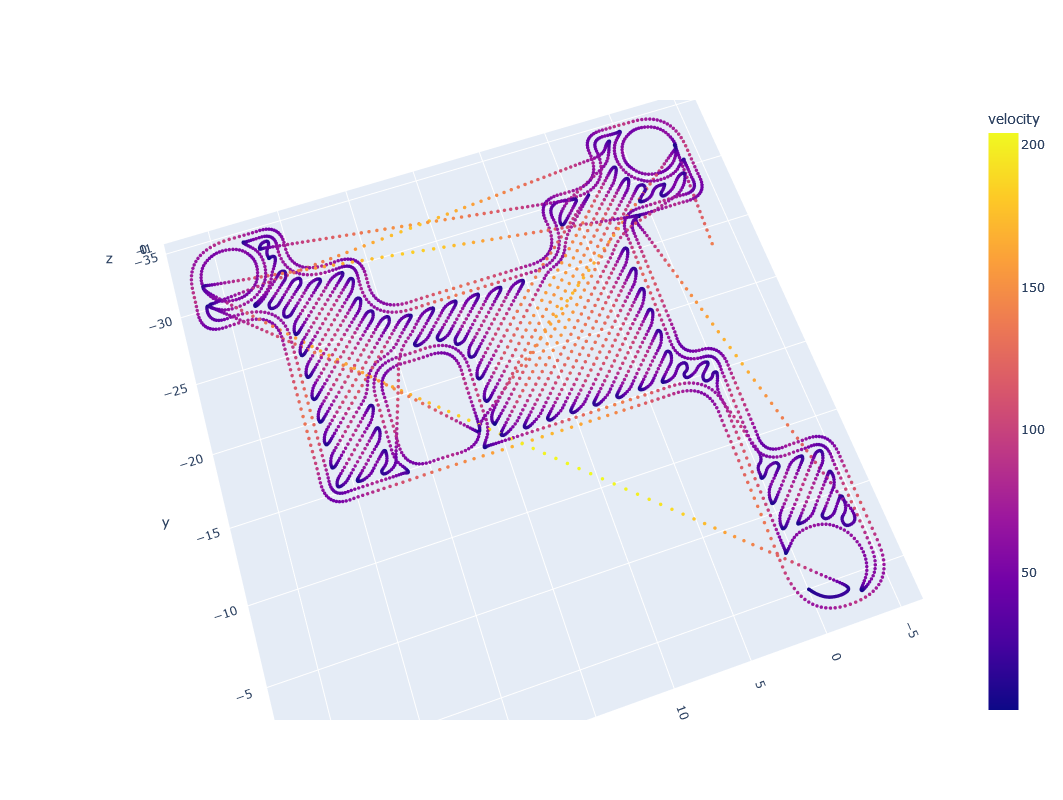
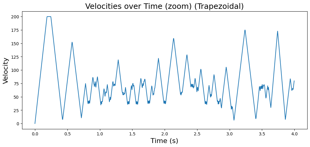
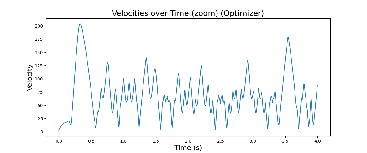
In Figure 6.13 and Figure 6.14 below, I show some early results of the solver operating on a motion system alone: because our solver can use a more nuanced motor model than off-the-shelf trapezoidal solvers, it manages a 15% increase in overall speed and produces a smoother velocity plot.
TODO: in these comparisons, what style motion are we comparing to ? does this mean waking up the trapezoidal solver again ? then show us what the two “models” look like…
6.5.2 Learning from Models
FIGURES: machines / motors, parameters learned, stiffnesses (from resonance?), and … where we can see each machine is most often limited, which motor, or when is stiffness limited and when is torque limited ?
6.5.3 Model Transferability
Also of curiousity is whether these models could be transferrable across materials or machines, or even processes. For example, it is likely that motion control models can be very simple and easily ported from machine to machine, but process models may need to be re-trained (or fit) for any new machine, material, or even for small changes of a machine (such as a nozzle diameter change or the ilk).
Basically this is going to be… that motor models are transferrable, and even a good source of truth, if we can i.e. deploy motors that are well understood, and then use those as measures of machine mass, transmission ratios, and frictional / stiffnesses etc.
6.6 Future Work
6.6.1 Generalizing Kinematics
… kinematic discovery from-scratch ? symbolic regression ? cameras ?
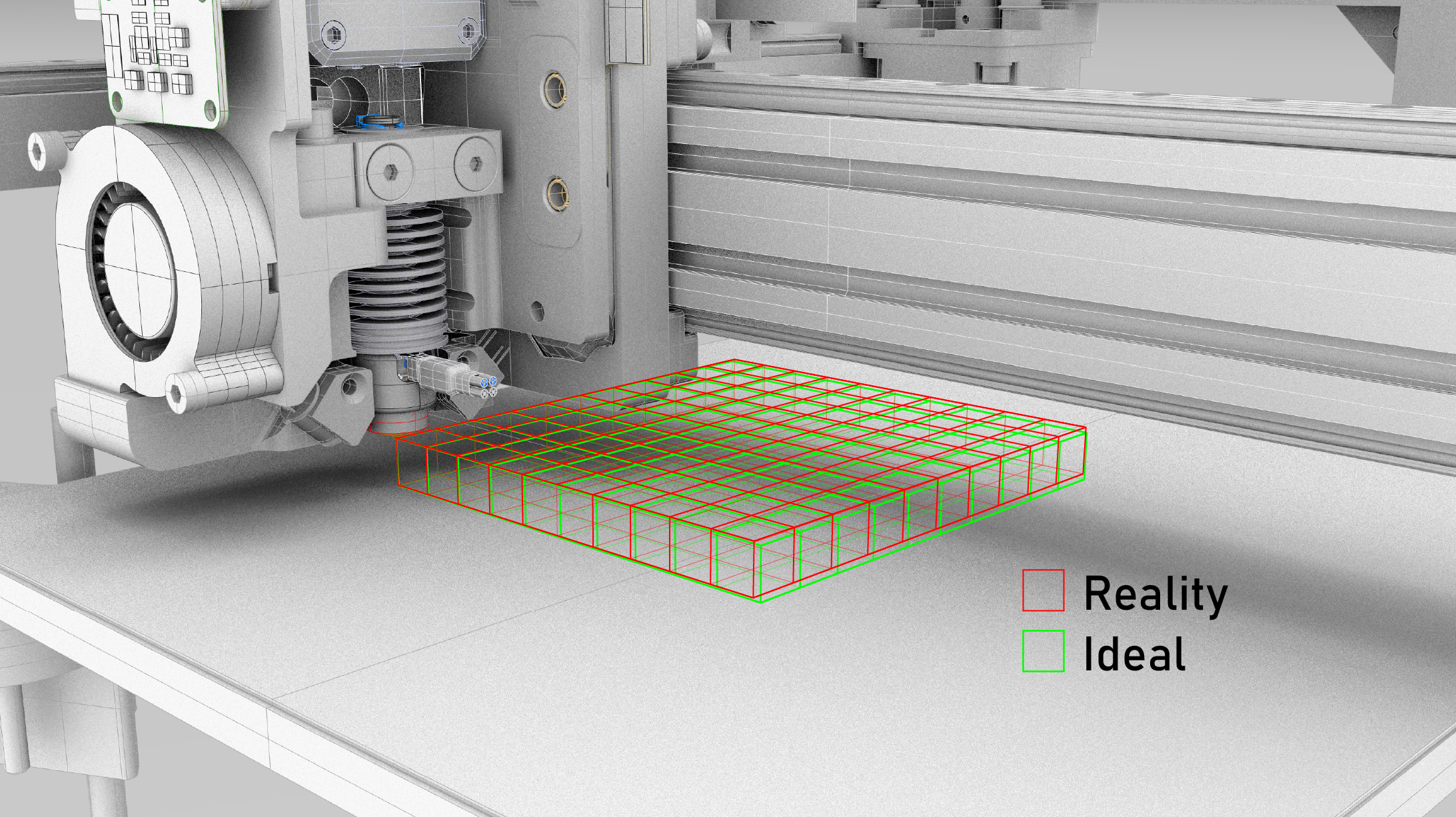
There is a lot that I didn’t get to on the topic of motion control. Probably the most frustrating of which is the task of more generally fitting kinematic models from motion data. The idea here would be that we could develop well known motor models, attach those to new machines, and automatically discover how they are configured vis-a-vis the machine’s transmission elements and mechanisms. This would be invaluable to machine builders because working out kinematic models is cumbersome first in getting configurations correct (motor offsets, transmission ratios), and then for refining those models: machines never go together exactly the way they are planned (no two lines are completely parallel, etc), and to achieve real precision we often need to fit kinematic models to data. For example the simple task of figuring out a machine’s exact working volume is often done with simple trial and error.
In some proposed schemes, we could develop a library of possible kinematic arrangements, attach an accelerometer to the end effector (as I have done here to work out resonances), and learn how each actuator’s acceleration corresponds to end effector motion. Backing out linear transforms is presumably as easy as filling in the matrix that relates one system to the other (see EQN (?)), but nonlinear transforms would also require that we guess the composition of the transform function and its inverse. Inprecise models like neural networks might get close in this regard, but are probably too much of a black-box to be truly suitable to the task: in machine design and control, it is invaluable to have precise definitions of our core systems.
Adding computer vision to learn kinematic models more concretely is another proposal (or hybrids of each), and my colleage Quentin Bolsee is working on this currently at the CBA. There are a littany of other data collection approaches for this task: probing known geometries (like the method outlined for bed leveling in this work) is a common one, and could be extended to correct for XY kinematics as well as in Z (as is in fact common on some 3D printers).
6.6.2 A Spec for Machine Digital Twins
One of the ideas that developed as I was working on these controllers is that of interfacing the (already software-based) controller to a “digital twin” of the whole machine. I think the most productive version of this idea is to use the digital twin as an interface between the machine designers’ understanding of their hardware’s kinematics and the controller.
FIGURE: little-guy, and printer digital twin
COMPARE: ROS Robot Description Language ?
For example we can normally take for granted that a machine designer will have a mostly complete CAD model of their output. Those CAD models are normally assembled using constraints that generate mechanisms: linear slides, rotary joints, etc - everything we need for a rigid body simulation.
A hope had been that we could develop a representation of these assemblies that could be exported from a CAD tool and plugged directly into the solver: the solver could then run and visualize the machine virtually to ensure that the designer’s idea of how the machine was going to move matched to reality. Data from motors could be used to verify and improve these alignments in all of the ways I’ve discussed previously. This representation could be as simple as a set of .stl or .step of the rigid bodies, and some .xml or .json outlining their relations to one another (joint types, etc), as well as linkages to actuators.
The goal of this tool would be to enable machine designers to quickly bring their machines to life, using a representation and interface (their CAD model) that they are already familiar with. Some such projects exist, i.e. ROBOT_XML (?), etc… yada yada - done well, the tool could also help machine designers learn about their designs’ performance before they build it, i.e. that a motor should be made more or less powerful, or a transmission element made stiffer, or that their mechanism could be improved to increase the machine’s range of motion, etc…
6.6.3 Composing Motion Systems and Automation
Another aspect that I wish I had been able to develop more completely is the idea of using graphs of functional blocks to compose motion systems. I originally spoke with Ilan Moyer about this idea some years ago, soon after I had realized that basis splines were a suitable representation for fluid motion4. The control points are so simple to transform (including through nonlinear transforms), since they alone are stateless: we can simply think of transforming position to position. However, we can also do transforms that change through time since they are continuously generated, i.e. applying an acceleration limit, etc.
More generally this some “flow of positions in time” that can be transformed arbitrarily, and it means that we can also i.e. record points, replay them, loop them, multiply them, add and subtract offsets, etc. This opens the door not just to better planning algorithms but to more abstract realtime control for tool-building: each transform block can be controlled by some other input: direct user controls, inputs from other motion systems, etc. Ilan came up with a lot of these ideas and has since finished some really excellent work, implementing it with a system that transforms step and direction pulses directly, rather than the more abstract basis spline.
The core principles should extend to make it possible to very quickly build automation more generally: conveyors, material handlers, etc: imagine all of the machines in a bottling plant. These are all subject to motion dynamics, but across “n dofs,” some of which are coupled but many are not. Graphs that contain motion flows and normal logic elements could be a really good framework for assembling their controllers.
References
Maths Vegetables is a Quentin-ism; oftentimes there are pretty well established mathematic solutions to the problems we face in machine control. The trouble with a maths education is that it can be boring when we learn it in the abstract. However, if we don’t eat those vegetables, we don’t understand the landscape of possible approaches when we get to the fun problems.↩︎
Actually, very many systems are actuated with hydraulics (heavy equiment) and pneumatics (factories are filled with pneumatic cylinders and valves etc). Hopefully by the end of this (and the next) chapter, you will see how the approach I present could be extended to suit these systems, but I am not going to get into it directly.↩︎
Decision Variables: i.e. the values that the solver picks.↩︎
I’m still not sure why I hadn’t figured the basis splines out earlier, it seems so obvious in hindsight. In fact I remember one summer at Haystack where I felt as though I had the gist of the idea: that we should be able to stream a simple stream of points at a fixed time interval, and do some local interpolation across those points. I think at this time I went looking for the right interpolation function, but failed to find the basis spline. I then fumbled around with awkward line segment representations for a year or so until the basis spline showed up somewhere and I realized how well it could work. I should say that the seed of this idea was given to me by Sam Calisch, who (when I was a masters student at the CBA) spoke with me about this idea of compressing generalized trajectories in some kind of elegant mathematic representation - he suggested it would be a spline of some kind, and again I don’t know why the basis spline wasn’t obvious. Maybe it was due to it’s not being a direct interpolation, which might seem like it disqualifies it outright were it not that the simple bandaid fix of transmitting very many points all the time made it suitable. Or maybe it is that the availability of embedded compute has changed drastically since even then. For what it is worth I also now know that splines are in fact quite common in motion control and robotics, so I maybe should have just done more homework.↩︎