5 MAXL: Synchronized Motion for Modular Hardware and Software
Modular Acceleration planning and eXecution Library (hah)
In the prior chapter I laid out a series of interfaces and tools on top of which I have developed the remainder of the applications in this thesis (and some others, and hopefully many more in the future).
Those tools let us connect software components throughout a given distributed system to one another across various networking links, and give us nice high-level handles on each of our components with which to do systems assembly - i.e. to turn those bits and pieces into some particular application (and many different applications using the same bits and pieces).
Critically for motion control, one of the tools in that kit is time synchronization. As we will see in this chapter, synchronizing clocks throughout our system is a key basis with which we can build the primary application that the thesis is interested in: the control of physical systems. Time sync not only lets us ensure that each of our actuators is in the right position at the right times, but also lets us create time-series datasets from modular sensors on the same machines that we can use to build and improve models (CH:next), which we can then use to do even better motion planning (CH:next->next).
Unfortunately for everyone involved, computer networks are never perfect. Any time we send a piece of data from one device to another, it takes some time to get there (delay), and requires some extra computing power to serialize, transmit, receive, route, and deserialize (overhead).
how much of this should be in the prior chapter ?
Network performance is also variable: if a link is congested its performance will decrease nonlinearly (i.e. slowly at first and then all at once) 1. Link performance is also dependent on “out of band” disturbances i.e. the electromagnetic environment. I was once debugging a packet loss issue for nearly half of a day before I realized that the cable (containing UART over RS485) was lying on top of a switching power supply, which was emitting noise in around the same frequency of the link’s bitrate. I moved the cable and the performance was restored. Wireless links are the same: too many cellphones in a room and your bluetooth headphones might stop working2.
All this to say that no matter how much engineering we do in our network layers, they will always be less performant and more importantly less deterministic than digital control (i.e. where all control elements are in the same CPU), because moving things into and out of a computer’s memory is always faster than shuffling it around on a network - except for when we are saturating that computing device’s available clock cycles (as is often the case!)3, in which case it is nice to be able to grow the system beyond one CPU and offload some tasks to other devices.
This poses what I have been calling the partitioning problem - given some distributed system (a machine, say), how do we split the requisite tasks amongst some set of devices (motors, sensors, and a coordinating computer, for example), such that we have acceptable and scalable performance. In the context of this thesis, I take for granted that flexibility is of primary concern: we want also to be able to make many different systems by adding and removing components from the mesh.
The contents of this chapter is a solution for the partitioning of generic motion control of many actuators and sensors in a distributed physical system. It is based on time synchronization between devices and representations of trajectory elements that are essentially functions of time which can be evaluated continuously, i.e. so that any device can measure it’s clock, put that time stamp into the function, and get back the value that it should be tracking at that time (and subsequently do whatever task is required to make that value a real world output).
In some earlier work (Read, Peek, and Gershenfeld 2023) I called these functions tracks. They are basically queues of various flavour that are explicitly encoded in time (rather than index, for example). They can encode position, velocity, levels (like laser power), events (like pulses to an injet head), or triggers (i.e. to tell a sensor when to read a value).
what is the value of this ? allude to… evaluation of this section ?
Encoding these in time is useful because it lets us remain synchronized in the face of variable or substantial network delay (i.e. we broadcast track control points ahead of time so that they are all realized in synchronous time). Tracks are also a convenient way to effectively compress time series information as a functional representation (more on that later), and to partition global states (the position of all motors at any \(t\)) into chunks (the position of a motor at any \(t\)). Perhaps most importantly, they let us put more intelligence into the edges (or knuckles (Section?)) of our systems, offloading some compute from the likely over-burdened co-ordinator. Time-series encodings (for example) would enable us to run smaller, local model predictive controllers in advanced use cases.
5.1 Common Approaches to Motion Coordination
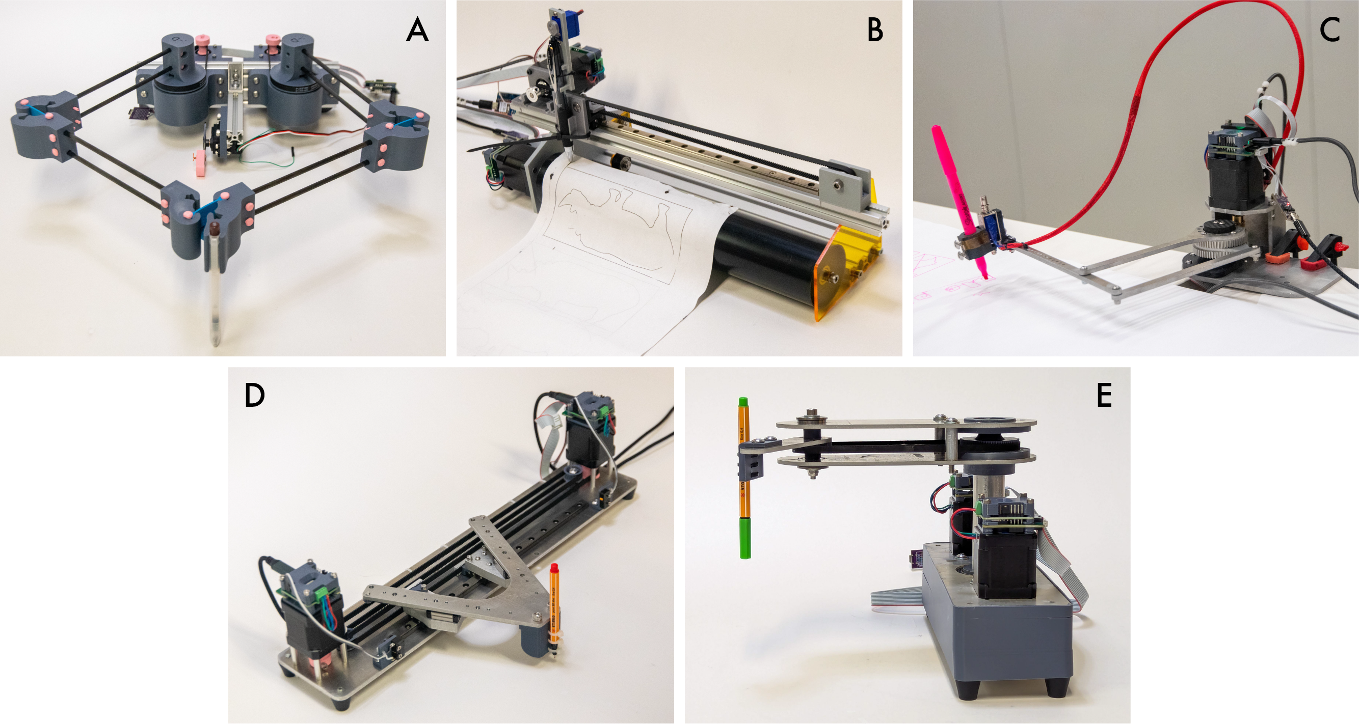
Of course I am not the first to develop motion control systems. I want to lay out three common architectures from industrial control to hobby 3D printing, and also discuss relevant work on flexible motion control from the CBA’s own community. Each of these solves the partitioning problem in differing ways, and each has its own drawbacks and advantages.
5.1.1 A Note on Hierarchichal Control Loops
From… brunton, or something? It is common to think about control problems as nested loops: top level (most complex)… each adding an order, until we get to ~ (basically) voltage controllers. These layers are natural partitioning boundaries…
5.1.2 Monlithic Control Boards
FIGURE: GRBL, Smoothieboard, and the Fab Light Controller ?
- monolithic control on some firmware eating gcode
5.1.3 Centralized Control + Servo Loops
FIGURE: DIN-mounted interpolator + ethercat (or similar) to servos,
- velocity loops, position loops… sample-and-hold control (introduces the constraint that lots of action needs to happen in one tight loop, which can be punishing and drives the use of expensive networking tech and bespoke computer hardware (i.e. realtime OS’es))
5.1.4 GCode’s Relationship to the Partitioning Problem
… architecture leads to the representations we use: these approaches are basically why we have gcode: this middle layer (where we have super-tight stuff going on) can’t provide arbitrary interfaces, needs to be buttoned down, and so we make GCode: we want to see if we can squish this out a little bit
5.1.5 Klipper
FIGURE: Klipper… a cool hybrid, we offload most smarts and do low level timing in hardware. Disadvantage is that is mostly-fundamentally based on step trains.
5.1.6 Gestalt / Object Oriented Hardware
FIGURE (?) and ref to Gestalt, Nadya…
- what does gestalt do ? honestly not sure how step trains are calculated and transmitted.
- a bus, python interfaces (similar!), but no device-to-device communication or pipes, not flexible across busses,
5.2 Background and Trade-Offs in Networked Control
delay, overhead, etc (as discussed, probably ?)
network determinism, realtime vs. soft-realtime vs (normal) systems, (pls clarify that even realtime systems just means that if something doesn’t happen in time, we trigger an error state: there is always the chance that someone cuts the cable…) trading compute for bandwidth (estimators, partial models…)
ease of development vs. performance,
a nugget on transaction cost economics ? networks, network ifaces actually very good way to partition experts and firms
5.3 MAXL’s Operating Principle
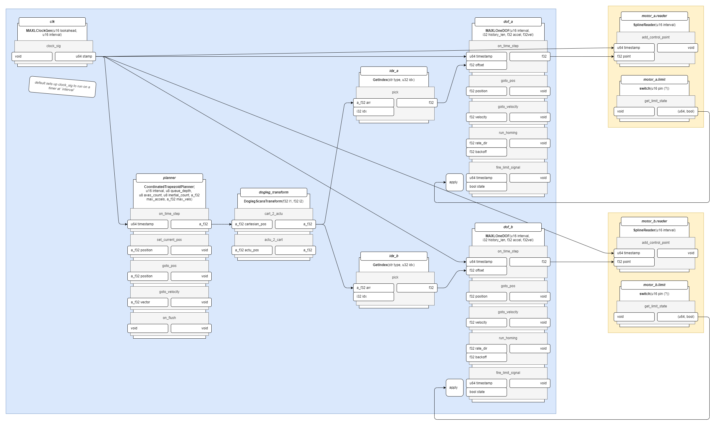
FIGURE: the basic overlay of the systems architecture… devices w/ time sync over links, and a graph including a clock source, pipes, transforms, and interpolators…
MAXL is a machine control framework that I have authored over the course of my time at MIT. It runs on top of the systems glue I have developed alongside it (OSAP, see Chapter 2) and consists of a few key components:
- Firmware libraries that allow embedded device authors to expose functionality to motion planners.
- Software libraries that allow machine builders to author kinematic models of their machines.
- Software libraries that allow machine builders to author optimization-based solvers for their machines.
MAXL’s contribution is to provide a generalizeable framework to control almost any machine using a set of re-useable software modules. It presents motion control systems as assemblies of functional blocks, where the aim is to allow machine developers to build controls systems from modules that are each easy to comprehend, but whose various combinations can span a large space of possible machine designs - as well as provide a proving ground for other systems described earlier in this proposal, like automatically calibrated kinematic arrangements, or model-based optimizations.
MAXL’s architecture is best explained with (FIGURE ABOVE). Graph configuration allows us to make application specific controllers (… the graph) with re-useable components. Each component block (a pipes (SECTION) class or function) receives a time stamp and a series of floating point values in something probably called on_new_point - each block can perform whatever logic it wants on the points (explained below ?), and passes new points to the next, or to an interpolator where they are evaluated as a basis spline (next section) track…
Operations on basis splines is more obvious, not sure if it is possible / if we want to explore transforms on other blocks, but presumably we can do any mixture of scaling, smoothing, squishing, transforming?
How do we write blocks (python codes) how do we configure them (python codes), and (future work) to instantiate and configure them in hardware.
5.3.1 Time Synchronized Basis Splines as a Fundamental Representation for Motion
Earlier in this section I introduced the idea of using tracks to coordinate motion and end effector outputs. The most useful and pervasive track within MAXL is a basis spline representation for motion.
FIGURE: the basis spline TODO: much of this is in _02_prop_results.md already
In particular, I use a cubic basis spline interpolation (often just called a B-spline) with control points (aka knots) at fixed time intervals. This spline (FIGURE, with example set of control points (LISTING)) is a piecewise polynomial that I’ve laid out in (LISTING). Basis splines are common in CAD and in computer graphics…
… I want to note that this idea has a long legacy; I had first discussed splines as a possible strategy with Sam Calisch, the motivation being much the same (I was looking for the answers to the same questions even back then) - how do we represent potentially complex trajectories (with nonlinear transforms, yada yada) to firmwares in a way that is extensible across machine types, motor types, and trajectories, but is also performant and small - in per-segment packet size and in computing complexity … and in a way that would not require us to re-program our motors when we make new machines. I spent a long time as well discussing this with Quentin Bolsee, whose contributions… and I have heard through various grapevines that “arbitrary spline-following” motion control is a kind of industry norm, but no-one seems to have written the details of all that down anywhere, so I am including it here for posterity and, more importantly, for the next of us who decides to write a motion controller.
I like the basis spline as a representation for motion because it has well defined and smooth derivatives for velocity and acceleration, with step functions in jerk. A plot at (FIGURE) shows these components of the spline laid out in (OTHER FIGURE), and (LISTING) shows the definitions for each derivative. The basis spline matches well to inertial systems controlled by electric motors because they have the same order. As discussed in (SECTION: MOTORS), our actuators cannot instantaneously change the amount of torque they are exerting, since it takes time for an applied voltage on the motor stator to develop into current (and so, torque / force). This means that electric motors cannot instantaneously change accelerations, although they can make instananeous changes to the rate of change in acceleration (i.e. voltage, jerk).
\[ P(t) = \begin{bmatrix}1 & t & t^2 & t^3 \end{bmatrix}\frac{1}{6} \begin{bmatrix} 1 & 4 & 1 & 0 \\ -3 & 0 & 3 & 0 \\ 3 & -6 & 3 & 0 \\ -1 & 3 & -3 & 1 \\ \end{bmatrix} \begin{bmatrix} P0 \\ P1 \\ P2 \\ P3 \\ \end{bmatrix} \tag{5.1}\]
Equation 5.1 is the cubic basis-spline form that MAXL uses. \(t\) spans a fixed interval, and the interval is set at some integer value of microseconds that is a power of two, between 256us and 16384us. Using these intervals means that the spline can be evaluated using fixed point arithmetic in embedded devices. Basis splines have the helpful property that we can always add new points to the end of a stream, meaning that at each interval we only need to stream one new position (whereas i.e. a linear segment of similar length would require much more information). This works well for motion because the splines’ own properties are well matched to moving systems (Holmer 2022). Fixed-interval tends to work because detail in motion tends to correlate to slower velocities (and so we end up packing more points in intricate parts of the path). While using these splines has been hugely productive for rapid machine development (their deployment means that I don’t have to modify motor firmwares in order to develop new motion schemes or kinematic models, etc). Splines are a lossy abstraction. They are not a direct interpolation, and at long time intervals they can result in motion that deviates from planned positions. I am overdue to carefully quantify these losses and their tradeoffs, and I should do so as I finish the PhD.
This is either trivial (if you do a lot of this kind modeling), or kind of confusing, so I made the figure (FIGURE_X) to line up (at left) motor controller states for applied voltage, current (force), velocity and position, and (at right) the same states from a basis spline whose control points are taken at fixed time intervals from the simulation of that motor - we can see the clear equivalence where jerk ~= voltage, accel ~= current, velocity ~= velocity.
5.3.1.1 Why Use Fixed Intervals?
… there are other spline representations, i.e. where knots have weights, where \(\dot{s}(t)\) is variable, etc, but I choose to use a scheme where each control point comes at equal time intervals apart, why?
- it means that directly picking x(t) off of any other representation and transmitting those is a (very ?) good approximation (for sufficiently small intervals) (see (SECTION BELOW))
- it means that evaluation is faster, since we know that
s(t) = 1always, - it makes for deterministic network loadings: we discussed earlier how variable data rates can be problematic… on issue that arises constantly in motion transmission is that we have big differences in data rates when we transmit i.e. line segments: in areas with low details (long lines) the rate is low, and then when we hit big detailed sections (i.e. a helical ramp), we suddenly need lots of bandwidth - this jumpiness is undesireable, and by sending always the same interval, if it works at all it will continue to work…
5.3.1.2 Quickly Evaluating Basis Splines in Firmware
Basis splines are great but evaluating them can require that we do lots of floating point arithmetic: about (X) floating point operations (LISTING) in total every time we want to evaluate the spline. In a motor driver, we basically want to be able to evaluate this as often as possible. The exact speed at which we do the evaluation is dependent on the system: in a low inertia servo drive, one to five kilohertz is enough, but with small inertias (that can change positions very quickly) we often want closer to 25 kHz. In stepper motors, we have to make a discrete step for any given position. Some stepper drivers have extremely fine discrete steps (51200 discrete ticks per revolution is not uncommon), meaning we want to evaluate the spline at closer to 100kHz. These rates can make for punishing numbers of Floating Point Operations Per Second (FPOPS) (see LISTING: MCUs, MHz, Rates, FPOPS @ Rate?).
LISTING: common mcus, costs, FPU availability, and equivalent FPOPS ? caption: yada yada… keep in mind that we also need headroom to do other stuff: i.e. use the evaluation LISTING: FPOPS per spline eval (w/ and w/o pre-calculating a…d,), and multipled by kHz evaluation rate
We additionally want to be able to evaluate these splines on cheap and simple microcontrollers (MCUs): one of the major downsides to modular systems is the increased cost for i.e. buying another microcontroller for each component in the system. Many of these devices do not have Floating Point Units (FPUs) (specialized bits of the MCU that let us do floating point arithmetic in one clock cycle). Where no FPU is available, adding or multiplying floating point values can take tens of clock cycles.
To ameliorate this issue, there are two steps we can take. The first is to pre-compute parameters a...d (lines x:y in LISTING) for given spline intervals once the relevant points are available. This saves time because these parameters are unchanging within one time interval - i.e. they only change every millisecond, whereas we might evaluate the spline every few microseconds. This reduces the FPOPS per evaluation down to (Y).
LISTING: the core spline evaluation step in firmware… floating point version
We can’t cut any more operations from the evaluation, but we can avoid floating point arithmetic in the cases where we don’t have an FPU. It may have seemed odd that the available time intervals for this spline are each some power of two (microseconds), but this is where that logic came from: with time as a power of two, we can more easily use fixed point arithmetic to evaluate the spline.
I should avoid going into a whole explainer on fixed point arithmetic, but the gist is that it lets us treat integer values in a computer as decimal values by declaring that some number of bits in each integer represent the value after the decimal place (and the rest represent whole numbers). For example if we take a 32 bit integer and say that the last 10 bits contain the value after the decimal place, we have a numeric resolution where one bit = 1/1024.
Microcontroller clocks are also naturally represented as integer counters, typically in an MCU we will have some function that we can call in order to get the number of microseconds that have elapsed since we turned the device on. OSAP’s clock synchronization service provides a similar function that we can call to get the number of microseconds since the system initialized - i.e. an integer count of microseconds that is synchronized across the network.
LISTING: the core maths again, fixed point boogaloo
So, taking our time interval of some power of two means that our conversion from time into the spline parameter \(s\) is exceptionally straightforward (line X in LISTING). From this point, the rest is just as easily re-cast to fixed point arithmetic, save for the normal fixed point gotchas (overflows, etc).
5.3.1.3 Even Fancier Tricks for Rapid Basis Spline Evaluation in Stepper Motors
As I mentioned earlier, stepper motors are the most punishing when it comes to spline evaluation, since we want to get close to 100kHz. Stepper motors make discrete steps, but motion is typically described as a smooth integration of velocities over time. There is a subtle piece of any stepper-driven motion system that translates between these two spaces (continuous and discrete).
In one common pattern, integration of velocity is done at a continuous clip (say, our 100kHz), to generate a new position at each interval. An additional counter is maintained in these systems: the displacement that has occured in the continuous system since a step pulse has been generated. This displacement is tracked in units such that 1.0 == one step - if the value rolls past 1.0 a step pulse is issued, and 1 is subtracted from that counter. If it rolls past -1.0, a step pulse in the other direction is issued, and 1 is added.
Other algorithms pre-compute step timings externally (i.e. Klipper, discussed in (SECTION)), or use Bresenham’s line algorithm (CITE) to calculate where along a line steps pulses should be issued.
With a fixed point implementation of the basis spline, it is possible to manipulate the splines’ value such that some bits in the output value correspond via bitwise logic to drive step pulses directly.
LISTING: how basis spline fixed point arithmetic can be arranged such that i.e. flipping the 11th bit means we need to generate a step pulse, and the 12th bit is our second (quadrature?) indicator for direction.
During my work at the CBA, I developed a strange stepper control circuit that drives a stepper motor using two HBridges, each of which has a current controller in hardware. In (SECTION: MOTORS) we looked at stepper motor architecture, so this should be familiar. In the driver I am discussing now (FIGURE), the software control loops from (FOC) are replaced with these HBridges’ chopper drivers, whose levels are set by writing to their VREF pins: for example, a voltage of 1.2v corresponds to a chopper driver setpoint at 2.0 amps … to drive the stepper, we send two out-of-phase current sinusoids out of these drivers.
FIGURE: the Simple Stepper board, and electrical / software flowchart…
The phase of those sinusoids corresponds to “microsteps” in the motor drive. To drive sinusoids, we can use lookup tables so that 0...16384 scales us from 0...2pi through the current phases. I have seen this now called “phase stepping” by others: rather than issue step pulses, we issue new stator phases at each update. This alone has the advantage that we can push our microstepping resolution to absurd limits without having to issues step pulses at obscene frequencies: if position deltas are small between updates, we make small microsteps, but if they are large (i.e. we are going fast), we make larger ‘steps’.
Perhaps you see where this is going w/r/t those splines: just like we manipulated our input basis spline scaling such that some of the bits corresponded to steps, we can do the same such that some window of bits corresponds directly to values in this lookup table that subsequently drive the stator currents. Is this still making sense? Try the figure, and its caption.
LISTING: block of code from spline -> rotor drive values -> hardware
This kind of bitwise alignment makes the job of evaluating the spline much less computationally intense, letting us push performance in simple devices. It is also numerically consistent and robust to the accumulation of small floating point errors over large timespans.
5.3.1.4 Using Spline Derivatives in Control
Servo drives work by tracking error between a target trajectory and their current position, using the error signal to set motor torque. This has the result that any servo will lag the control signal by some amount, since we need some error to appear before we begin controlling the motor. Normally this error can be kept very low by using large feedback gains. However, it is even better to be able to incorporate some feedforward gains in a control loop. Well tuned feedforward gains mean that the feedback path in the servo drive only has to accomodate for disturbances and modeling errors.
The most straightforward way to use a basis spline for servo control is to take the spline’s position and track that against the servo’s current position. The spline gives us velocity and acceleration in time as well, so we can add feedforward gains for these terms. For example, we know that the torque required to overcome friction in the system is a function of the velocity, and the torque required to produce a certain acceleration is a function of the system’s mass.
LISTINGS: feed-forward terms (are in motor_gains_smarts.ipynb)
We can of course only use these terms when we have good system models, and they can be detrimental when models are mismatched. However, in cases where they are well matched, their addition can reduce tracking errors.
FIGURE: servo traces w/ and w/o feedforward gains ?
The availability of these additional states also enables the development of more complete LQR controllers. I won’t go into details on this topic here, but LQR is fairly well understood, I merely want to point out another advantage to using basis splines in motion control.
5.3.1.5 Using Local Lookahead
For a final note, queuing motion as a function of time also opens up the possibility of using smaller lookahead controller within each device. As we drive performance of our motor drivers in the future (and continue to develop better models of these systems, and more embedded compute performance), using small Model Predictive Controllers for lookahead may become more prevalent and common (at the moment most practical controllers are simple PID loops). These require that each device has a future window of control commands to inspect, and time-encoded basis splines will be a useful representation in these cases.
In even simpler scenarios, some devices have known (and constant) lag times between actuation and output: for example an electromagnet or solenoid driven at the same voltage will always have the same delay (between when voltage is applied and when the target current is reached). Devices with fixed lag can simply inspect their target trajectory that many milliseconds in the future, and begin actuation ahead of time in order to delete lags.
5.3.2 Assembling MAXL Systems using Dataflow Blocks
“to provide a generalizeable framework to control almost any machine using a set of re-useable software modules…”
for example the solver (discussed next) goes in as one of these blocks: this un-burdens it from having to do i.e. limit switch homing, bed leveling, yada yada… we can also drop in a more classical trapezoid based solver for simple systems that we understand well, …
- developing motion controllers as dataflow graphs:
- using control points lets us do simple transforms on each point,
- we can chain… offsets, transforms, corrections, etc,
- using one system-wide timer and time sync…
- rpc on dataflow blocks for high-level operation of the flows, i.e. homing w/ the one_dof…
- distributing end-effector targets with
- basis splines (the same, very flexible)
- simple step-functions
- bitmasks of the same (inkjet)
- using distributed info. as targets for lower level controllers (loadcell following knife pressure, position as target / reference for motor (rather than feed-forward, simple))
Blocks Diagram for FFF w/ Optimizer, Data Collectors, Etc
5.3.3 In-Firmware Safety Backstops
- spline-safety backstops
- motion controllers developed by non-experts or in experimental schemes may generate busted outputs,
- networks are never 100% reliable (important footnote: a system’s being certified
realtimedoes not mean that it never errs, it only means that when it errs, safety flags and routines are triggered), and we will occasionally miss a packet: consider a 24hr long mfg job w/ time stamps 512us apart: we have (one large number) of packets to transmit across many devices, how many sigmas req’d to have zero errs ? - motors can each run very simple max-jerk computation: each incoming point is subject to this limit and if it lies outside of that point, we replace incoming point with that limit…
- selectable: max accel, max accel as function of velocity, max jerk as function of velocity (?) quick to compute…
5.3.4 Event-Based Tracks
besides splines for motion, we can implement ‘level’ and ‘event’ tracks
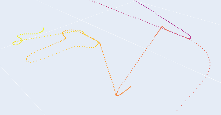
are slightly less composable FIGURE: add the light painting figure to show that we implemented this, to cover other events…
5.4 Time Synchronized Sensing and Data Collection
… just to say: we have pipes + timers (or event tracks), and sampling w/ stamps means that we can make time series (more later) (is not exactly maxl per se… but is, also ?)
- the basis in time sync… allows us to reconcile measurements with trajectory,
- (ref next chapters) having time-sync allows reconciliation of sensor data with trajectory states
- (as in the flow-model data gather, for example)
- (as in recollection of states during a print to make a digital twin of the part’s thermal history)
- (ref next chapters) having time-sync allows reconciliation of sensor data with trajectory states
5.5 Deploying MAXL Motion
- light painting or inkjet printing, for time-sync utility demonstration ?
- gigapan / surface scan for the same
- knife-pressure tool as an example of mixed closed / open loop work
5.5.1 A Plenitude of Machine Kinematics
MAXL… blocks allow us to mix kinematics w/ solvers, yada yada ?
And do i.e. recombination of software modules, as in bed mesh leveling where we can (1) re-use homing rountine to get tap posn’s, and (2) use a level’er block to apply corrections…
FIGURE: MAXl flow blocks for this bed correction…
5.5.2 Collecting Time-Aligned Data
My control approach requires that machine and material models be fit to the particular machine they are deployed on, and this means that MAXL and OSAP need to enable us to run data collection routines. It also involves the development of those collection routines.
FIG: i.e. show traces / outputs from solver, compared to data -> like, all of the printer outputs are this.
For this task, I lean on OSAP’s time synchronization and generate time-stamped data streams from sensors embedded in the machine. These let me generate detailed time-series datasets that are reconciled to the machine’s real motion trajectories. Those can then be used to fit models, using optimizers not dissimilar to the one which is used during online control (i.e. gradient-based search).
5.5.3 Basis Spline Precision and Performance
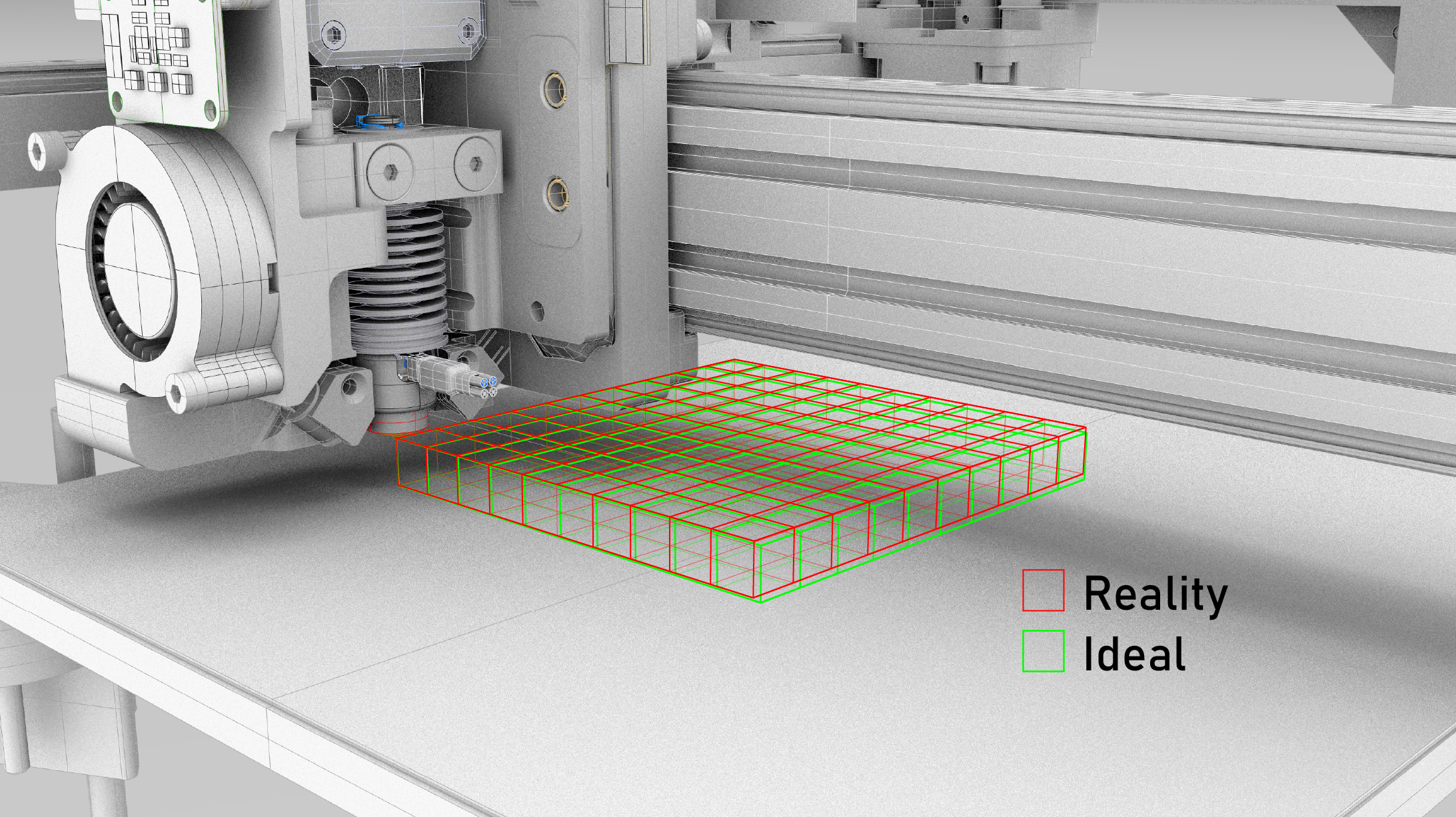
Earlier I was discussing how basis splines in MAXL are basically a compression / encoding that works well for “things that move” since they (basis splines and moving things) have the same order. One of the downsides of this encoding is that the compression becomes lossy when the spline’s control point intervals are not sufficiently close together in time.
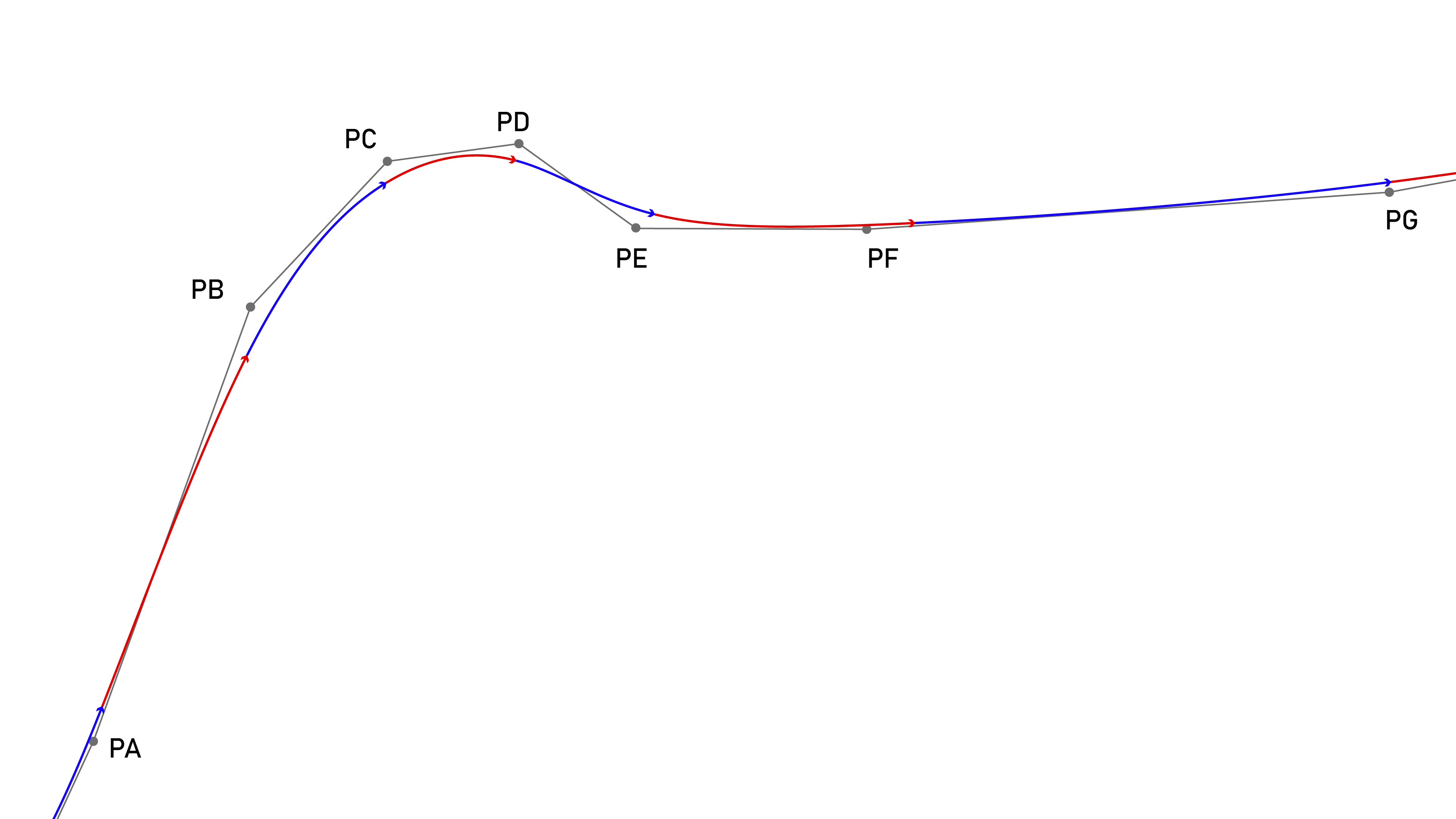
Basis splines are not a direct interpolation; points on the spline are not guaranteed to go directly through control points, as we see in (FIGURE_X). The displacement from the control point itself to the point on the spline at the same time we can call \(\epsilon\), which we can calculate here.
LISTING: \(\epsilon = sqrt(pt(t)^2 - spline(t)^2)\)
This displacement is zero when we are interpolating a straight line, but nonzero when we pass through corners. When we do so, its size is dependent on the speed with which we traverse the corner, the corner’s sharpness, and the spline’s time interval. To illustrate, let’s look at a 90’ corner traversed at 100mm/sec with control points generated every 2048us:
FIGURE: spline epsilon figure
On a first pass, this might seem unacceptable. However, the commanded motion is unrealistic: no inertial system can actually pass through this corner at 100mm/sec, as it would mean driving an infinite acceleration at the junction. Instead, our input trajectory is going to slow down as it approaches the corner, and speed up as it departs. If we make the same figure, but apply junction deviation to calculate a minimum cornering velocity, and apply accelerations into and out of that corner velocity, we see a very different result:
FIGURE: same, but with jd / accel,
As we can see the error drops significantly here, and becomes even more favourable when we interpolate faster, at 1024 us:
FIGURE: same, with 1ms interp…
All of the systems we are interested in controlling have this property: in areas with tight geometry, we tend to be going much slower than in areas with open geometry. As a result, our control points naturally bunch up in areas where there is more to describe, and so the compression tends to serve well, even though there is some loss.
In designing motion systems that use basis spline interpolation, it becomes important to be able to quantify this loss to find the interval size that will deliver suitable performance. To do so, honestly not sure yet, do other work above, then figure it out?
- can we generalize to curvature (radius), max speed @ curvature = acceleration, and look at error across radii for given intervals ?
References
Networks tend to collapse when they approach their maximum utilization. The typical pattern is that increasing congestion starts to cause packet loss, after which transport layer algorithms begin queuing extra messages (retransmits), further increasing congestion. Once everyone starts doing this, links are quickly saturated and performance bottlenecks. Much work has gone into developing transport algorithms that intelligently avoid and recover from these scenarios, i.e. (that sick paper on networks as distributed optimization), and i.e. TCP New Vegas (which uses packet delay, rather than packet loss, as a flow-control signal).↩︎
Believe it or not, microwaves (like, for cooking your freezer dinner) emit radio waves near 2.4GHz (the same band as WiFi) at obscene power levels (1.5kW, whereas your laptop’s WiFi transciever will use about 100 milliWatts). If you run a network speed test and then reheat your coffee, you might notice that link speed degrading…↩︎
Of course this is only true when we are not saturating that device’s compute power - which is actually often the case. In this work, the motor controllers are using all of their available 200MHz to servo the motors around. If we tried to stick the motion controller in there as well (and more motors), things would explode. This is additionally true for compute in general: datacenters and supercomputers rely on networks to expand compute volume beyond what is available on a single die.↩︎