7 Model-Based Control of an FFF 3D Printer

In the previous chapter I explained how we can optimize a machine trajectory using models of the machine’s actuators, kinematics and stiffness. I showed how model based trajectories are faster, smoother, and are automatically aligned with the physical hardware they are running on. In those cases, “optimum” simply meant “fast and precise.”

However, motion is only half of the story for most digital fabrication machines. On the other side we have process control, i.e. the flow and deposition of molten plastics in Fused Filament Fabrication (FFF 3D Printing), chip formation and resonance in CNC Machining, or laser / material interaction in a laser cutter, etc.

Getting a machine to work properly requires that these two aspects of control be considered simultaneously: if we have a flowrate limit in our FFF printer, and a track of a certain width and height, this corresponds to a translational speed limit. Flow from an FFF extruder is also nonlinear and history dependent: before extrusion begins, the extruder motor must generate pressure in the nozzle, and as a machine slows down, this pressure must be reduced in anticipation of the change in speed in order to maintain the same volumetric flow per mm of travel. From the previous chapter we understand that any machine has acceleration limits related to the machine’s mechanism, but the process can also impose acceleration limits: i.e. the extruder motor and filament have all the same dynamics as any other actuator, but are coupled through this pressure and flow model. Things can get complicated!

Figure 7.1: The physics of 3D printing is simple in principle (heat, then squish filament out of a nozzle) but can be complex in practice. Filament between the drive gears and nozzle exit compresses before it extrudes, putting some phase lag in the system. The amount that extrudes is a function of the chamber pressure, but also of the flow temperature and material properties. The actual flow temperature is history dependent: if we have been extruding near the machine’s limit, melt flows are normally colder than the nozzle’s measureable temperature (since the filament does not spend much time in the heat zone). To add to all of this, filaments exhibit *die swell* - when they are extruded at high pressures, they retain some memory of their previous width (as a 1.75mm diameter rod) and try to expand back to that width as they cool, putting residual stresses in the print.

In SOTA machines, these processes are modeled intuitively and tuned heuristically when users select parameters in CAM softwares that are used to generate GCodes to send to machines. I started discussing this in Section 1.2 and Section 1.3; CAM tools essentially give users control over the machines’ low level instructions, rather than helping them to understand the two physical systems that are under their control (the motion system and process), and how they relate to one another. As a quick example, it is possible to double the layer height for a 3D printer (doubling the required flowrates throughout), while keeping all of the selected translational speeds identical. This requires that the user intuit the fact that their changing the layer height doubles all of the flows being requested from the extruder and make the appropriate changes in other parameters in the system.

Low-level parameter tuning can work well for systems that are well understood but it means that bringing new materials and machines online requires many hours of hand tuning. It also means that parameters which are ultimately used may work but are not guaranteed to be optimal: we may find flow parameters that work well in most cases but fail in others, or which lie below the machine’s real capability.

In this chapter, I develop an FFF 3D Printer with some sensing equipment added to the extruder. Using this hardware, I generate models that let us simulate polymer flow given a time series of nozzle temperatures and extruder motor velocities. We can use these models alongside a small set of heuristics to pick high level operating parameters (like nozzle temperature). We also add them to the optimizer from the previous chapter to perform a combined optimization on the flow and motion dynamics.

Doing so reframes manual process tuning as model development. This means we can automate much of that trial and error. More importantly, it also teaches us about the hardware: models themselves are descriptive of the physics we are trying to control, and outputs from the solver tell us which components of the system are limiting or enabling performance at each point in the trajectory.

7.1 FFF CAM vs. FFF Phenomenology

Figure 7.2: A screenshot of parameters available to tune an FFF print job, from PrusaSlicer (P. Research 2024). The set which is displayed is incomplete; there is another page of parameters for extrusion temperature, print cooling fan settings, and bed temperature.

TODO: avoid repeating what was said above.

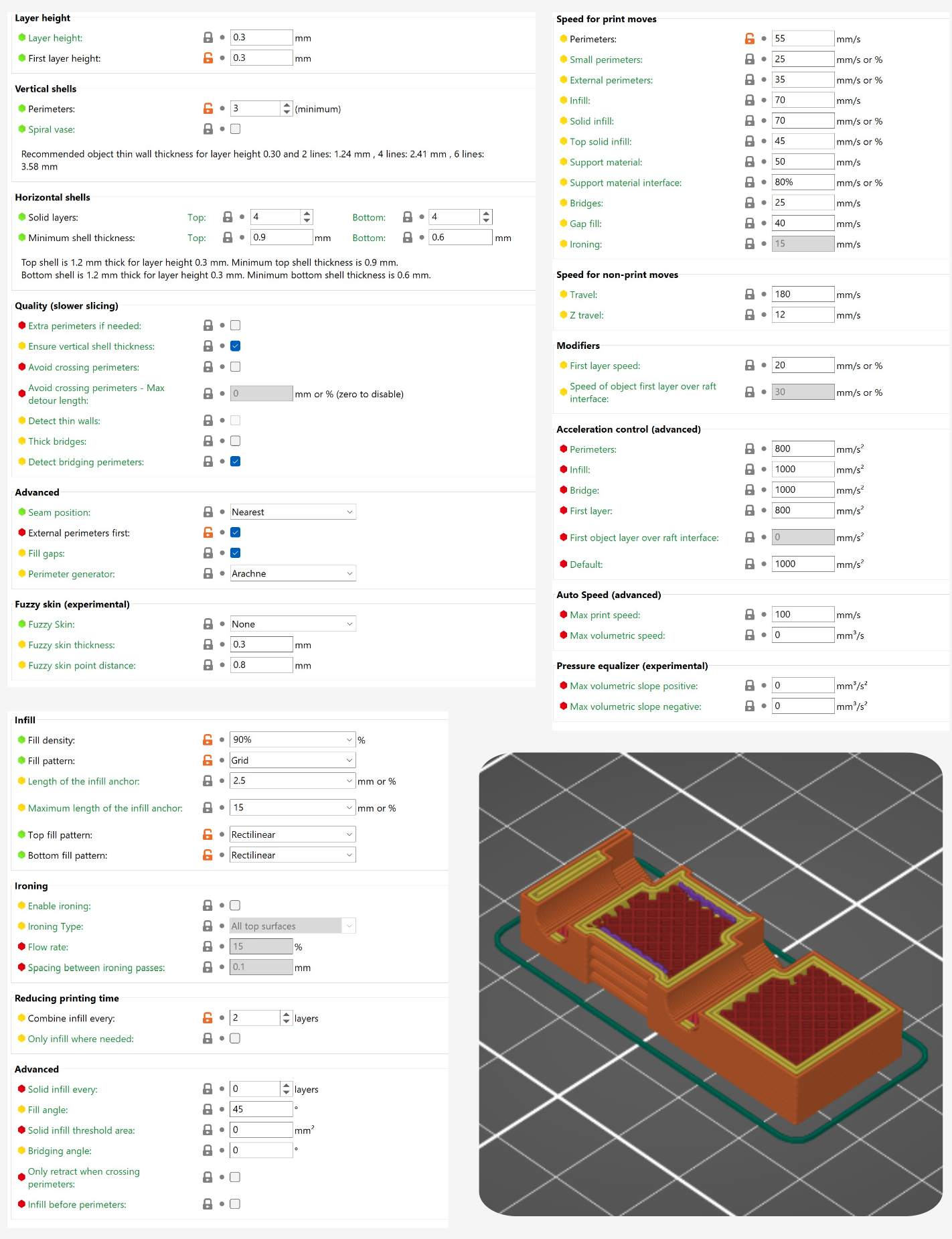
In CAM tools for 3D Printing (known as slicers) users import 3D objects and set parameters to tune the process. Some parameters are geometric: layer height, track widths, external perimeter counts, and infill pattern and density. Other parameters set the machine’s speed (how fast the nozzle moves in cartesian space, also called translational rates) for different features: outside perimeters, interior perimeters, infill, etc. They select temperatures: for the nozzle, for the print bed, and (sometimes) for the print chamber. Finally, they adjust cooling parameters: slicers maintain a minimum layer time with the goal that when the next layer is printed, the previously deposited material is solidifying; this is important to avoid print slumping. All told, there are about one hundred parameters to tune in a slicer. Many of them need to be tuned for each new material, and more need to be tune when we change i.e. the nozzle diameter. Historically, tuning these parameters was a major barrier to the adoption of 3D Printing, but the community has over the years developed good presets for most commonly available materials and printers. It still poses a challenge when we expand our material selections or build new hardware.

TABLE: print parameter groups, descriptions, relations to physics / comparison to how the same values are determined in this work. Note that i.e. speeds in slicers != speeds in reality in any system.

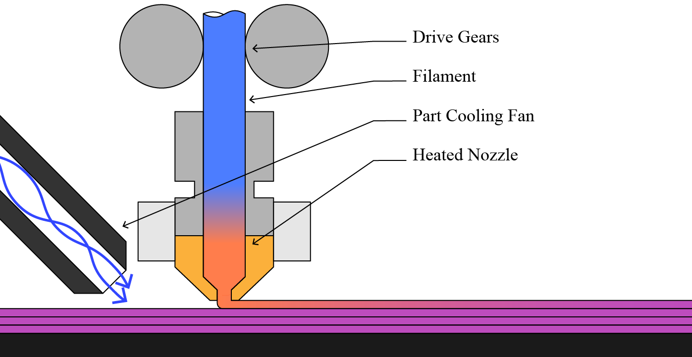
The values we set in slicers all relate explicitly to the machine instructions (how fast to travel, how thick to make the layer, etc). They relate implicitly to the physics of 3D printing, which has mostly to do with flow rates and temperature of the polymer melt (see Figure 7.1 above) (Mackay 2018). For example if we double the layer height but retain the same speeds we double the flowrate of the polymer melt: this has huge ramifications for the physics of the process, but that is not reflected anywhere else in the parameter set. Manually changing print speeds to reflect the new layer height would mean updating six other parameters (excluding those that can be set by a percentage). Nor are those parameters related to longer-term outcomes like the resulting thermal history of the print’s inter-layer joints, which are a main indicator of part strength (Coogan and Kazmer 2020). Inversely, if we increase the nozzle temperature we often unlock more flow rate, but there is no way to update print speeds as a function of temperature, or increase layer cooling time. Instead of having any knowledge of print physics built into the slicer, users need to intuit how these many parameters will relate to the machine’s operation.

7.2 The Rheo Printer

The Rheo Printer is an FFF 3D printer that combines much of the work discussed in this thesis. It uses online instrumentation to build models of its own motion systems and process physics, and then deploys those models in a controller that combines motion optimizations with process optimizations in one online loop. There are a few distinct contributions / results of note in this project.

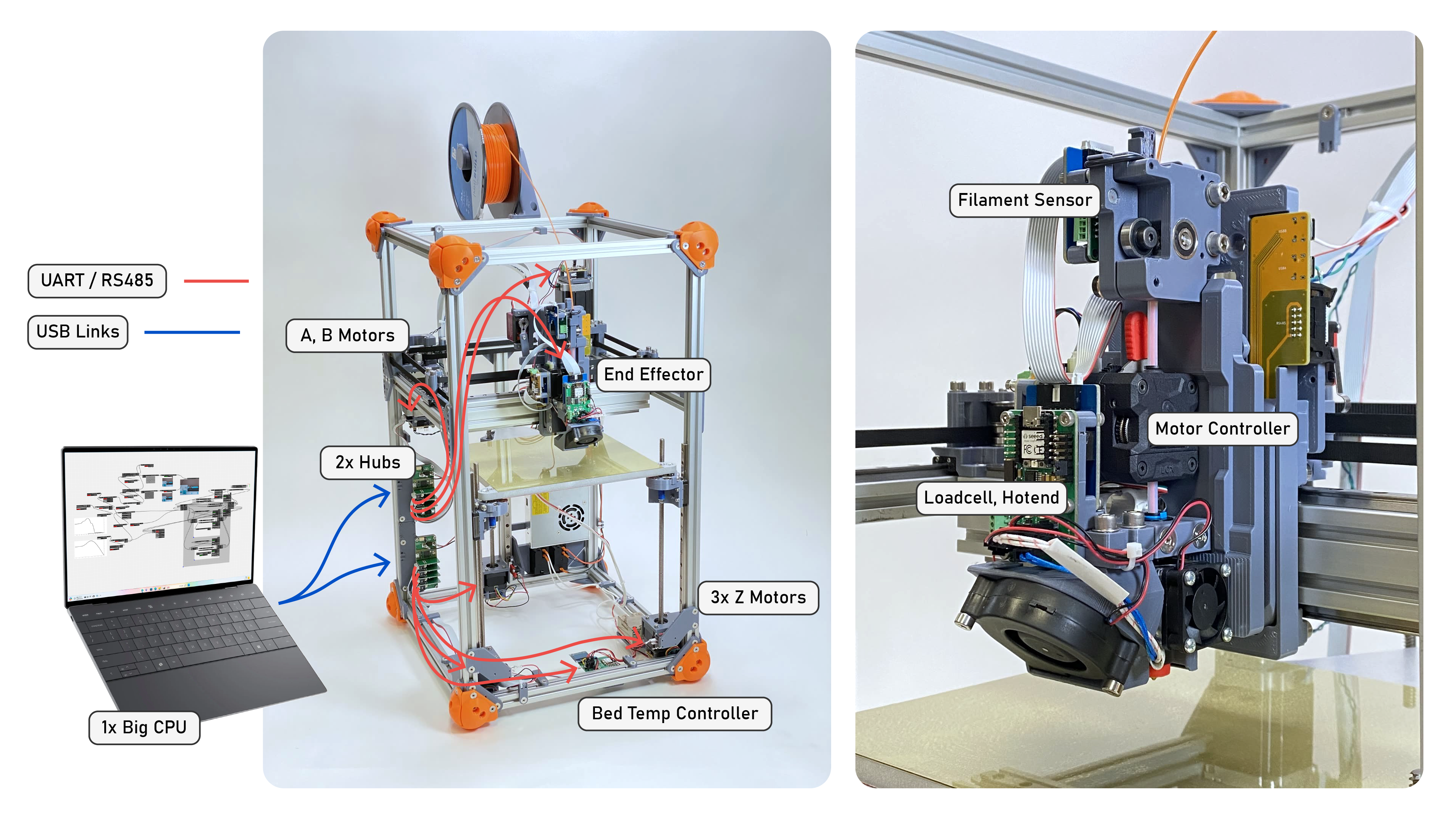
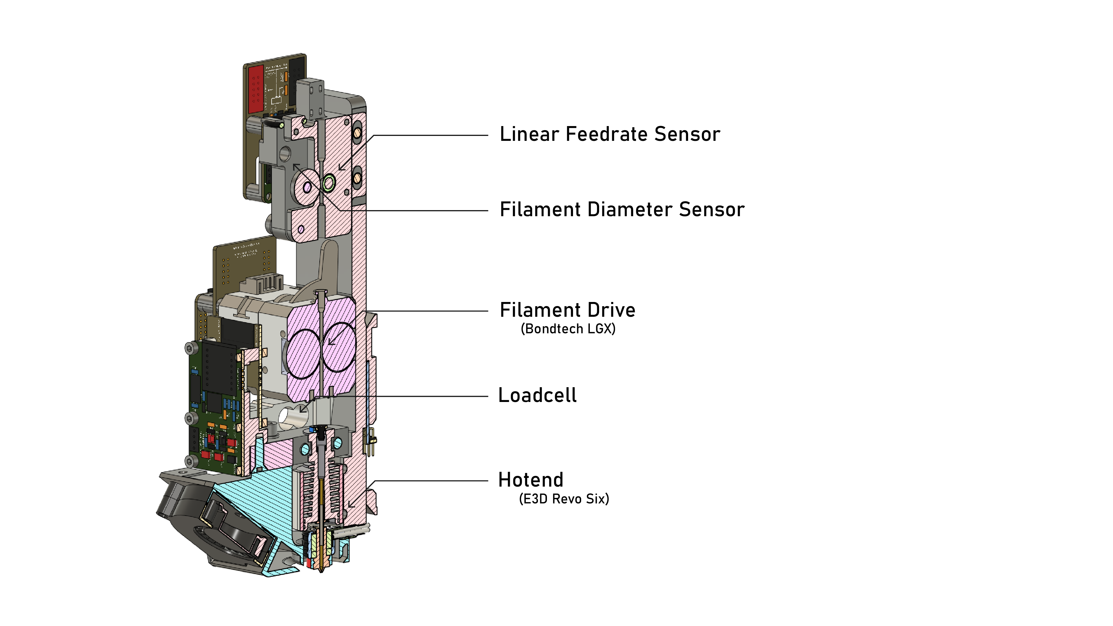
Figure 7.3: The Rheo Printer is an FFF 3D Printer that deploys the controllers I have developed in this thesis, and includes instrumentation for flow- and motion model building. Here I roughly diagram the controller’s physical layout: we use a PC to control the machine at a high level via OSAP, Pipes and MAXL. Controls are overlaid on a series of modular circuits embedded in the machine.

The Rheo Printer’s hotend features a loadcell between the hotend and extruder motor (which allows us to measure nozzle pressure), and a filament sensor that measures linear flowrate as well as filament thickness. The controls are assembled from modular electronics and connected using OSAP, controlled using MAXL.

The Rheo Printer’s hardware is representative of most commercially available FFF 3D Printers, except for the addition of instruments in the hotend, as detailed in the figure above.

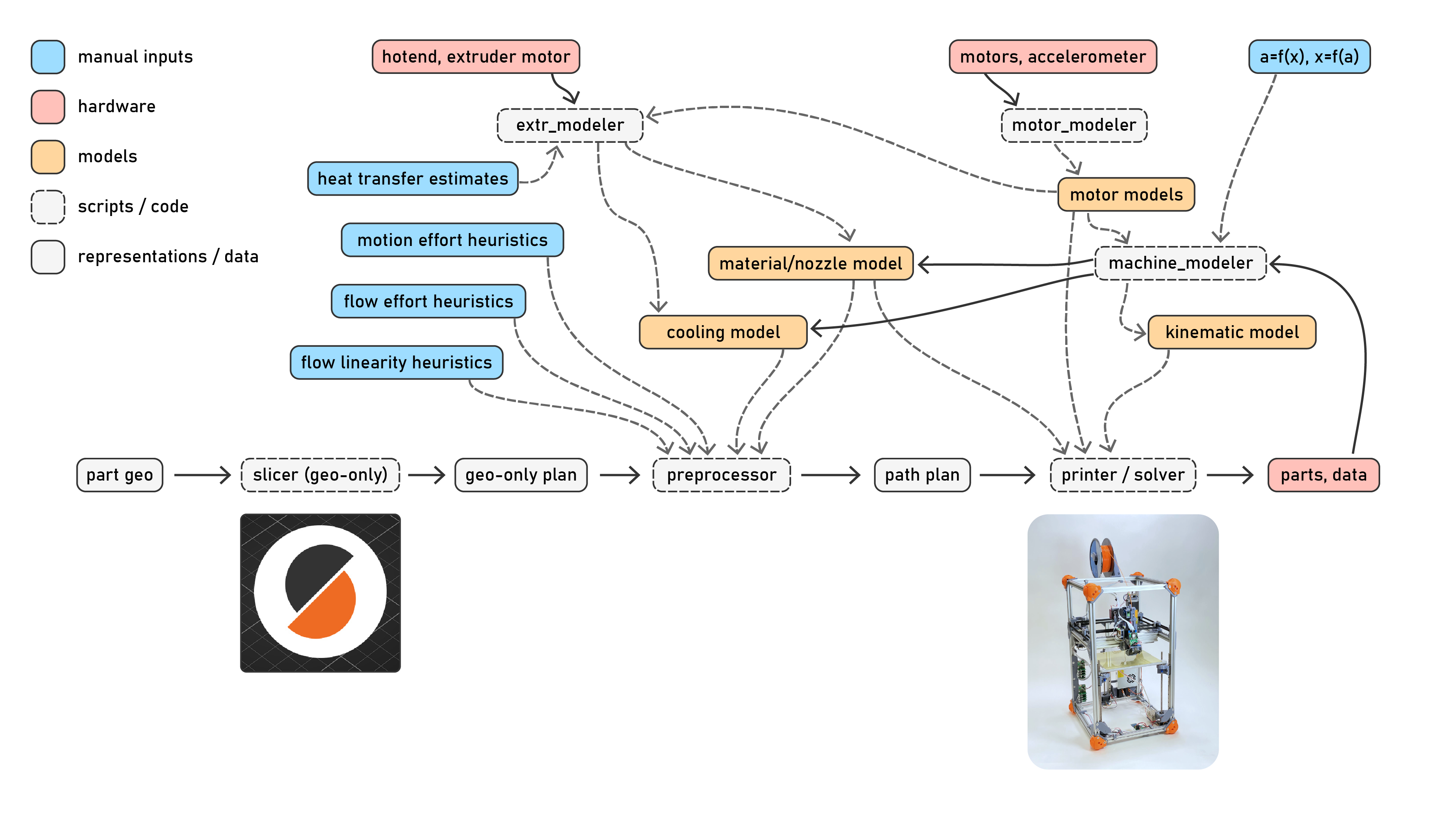
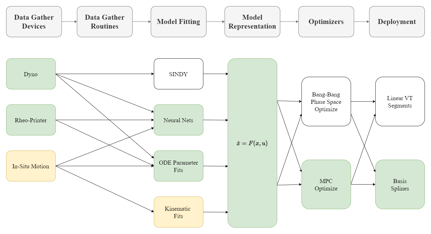
Figure 7.4: A systems level diagram of the Rheo Printer, articulating which devices on the machine generate which models and how those models are used across workflow components.

Since the Rheo Printer runs on models, the workflow is different than what users of off the shelf 3D Printers will expect. I diagram this above in Figure 7.4. To start, I make motor models for each actuator, as outlined in Section 6.1. Once the motors are mounted to the machine, I build a model of the machine’s kinematics terms: inertias, damping and stiffnesses per axis (Section 6.2, Section 6.3). This set of models doesn’t change during the lifetime of the machine, although they can be updated if hardware degrades, as I discuss in Section 7.7. For each new material, we fit a flow model: doing so consists of a steady-state test and a dynamics test (Section 7.3). Together, these tests take about 30 minutes, after which flow models are saved to disk. I should note that we need to fit a new flow model for each (material, nozzle) pair, i.e. if we have a model for PLA that was generated using a 0.4mm nozzle, but swap to a 0.6mm nozzle, we cannot adapt the PLA measurements to a larger nozzle. This is because the models are not “traditional” rheological models: we do not extract real values for viscosities, pressures, etc. ((Jake?): worth more discussion… is ‘computational metrology’).

Once we have collected all of our models, running the machine follows a somewhat familiar workflow. I use an off-the-shelf slicer to convert 3D models of parts to paths, in a geometry-only mode. Path segments are categorized as perimeters, infill, etc. I then run a pre-processor on this path that uses the flow models (and a small set of parameters) to select flowrate targets and nozzle temperatures. I outline that component in Section 7.4. Finally we send this data to the solver, which runs the machine in real time using flow and motion models to generate motor commands. In contrast to Figure 1.3, we can see that this workflow uses a substantial amount of feedback from the machine.

I should also point out that the machine continues to generate data while we are printing. Later on, we can use these data to fine tune our models or to expand them, for example using the parts measured thermal history to learn about it’s relationship to layer bonding, etc.

7.3 Polymer Flow Models for 3D Printing

To my immeasurable dissappointment, polymer extrusion is a deviously confounding system to model. See ?fig-extrusion-explainer (and caption) for an overview of the system. In total, probably one or two years’ worth of work in this thesis was done only on this topic: trying to understand it intuitively, and then trying to build fitting routines and mathematic models of that understanding that would suitably fit to data, and which are robust and simple enough to use as control components.

Big Extrusion Model Explainer, w/ labels matched to eqn labels…

Figure 7.5: What is each part of extruder called, what are relevant params, values, states…

Fundamentally we are trying to understand what flowrate will emerge from the tip of the nozzle at any given time (I will use \(Q_{out}\) for this value, in \(mm^3/s\)), at any given nozzle temperature and pressure. The value depends on a handful of inputs: (1) the polymer has a viscosity that is dependent on it’s temperature and shear rate (i.e. nozzle pressure: polymers are non-newtonian in that they are less viscous under higher pressures, more on that later), (2) the polymer between our motor and nozzle is compressible, and so we must build this pressure before extrusion begins (meaning our motor needs to begin pushing filament into the melt zone ahead of the time we want it to emerge), and (3) the extruder motor has its own dynamics, discussed earlier. Finally (4) the thermal history of the filament in the melt zone should be considered: filament in the melt zone takes time to come up to the nozzle’s temperature: at high speeds, the melt flow does not reach this temperature before it is extruded, leading to colder flows where we need more pressures to achieve the same flowrate.

So, in this section we will discuss finding steady state relationships between flow, pressure, and temperature, and then dynamic relationships for the same (including filament compression). We will then look at how we couple motor dynamics into this model, and finally look at the thermal data we can gather, its relationship to cooling and minimum layer times, and explore non-isothermal flows briefly. In the end, we will have robust models that we can fit across many filaments and machines, which can be used to generate control parameters and controllers.

7.3.1 Existing Research on Modelling FFF Polymer Flows

Luckily there is a lot of interest in FFF printing in the literature, and so the applied physics are quite thoroughly understood (Turner, Strong, and Gold 2014) (Mackay 2018).

Of particular relevance to this work is a line of research begun by TJ Coogan and David Kazmer, who developed an instrumented extruder similar to ours in (Coogan and Kazmer 2019). Filippos Tourlomousis takes credit for bringing this idea to the CBA and implementing the first version of the hardware, and I extend a design pattern developed by an FFF youtuber to implement the filament sensor (Sanladerer 2021) (adding a feedrate encoder, and calibrating width measurements). Kazmer continues work to characterize the dynamic behaviour of filament during extrusion in (Kazmer et al. 2021), which helped me to develop the dynamics model I use in the current iteration of the FFF flow model. These works were also fundamental to my work in (Read et al. 2024) (see Figure 7.9 and Figure 7.10), where we combined online model-building with parameter selection in a reduced space to print with unkown materials.

A selection of the literature disccusses performance limits to FFF printing, notably (Go et al. 2017) discusses absolute limits to print speeds based on nozzle thermodynamics and (Mackay et al. 2017) models flowrates through a hotend as a function of nozzle temperature. The focus of the work in this thesis is not necessarily to push those limits, but to develop controllers that more routinely run at or near those limits (pushing performance of existing systems).

Another selection studies the relationship between slicer settings and print performance (strength, precision) (Afonso et al. 2021) (Deshwal, Kumar, and Chhabra 2020) (Qattawi et al. 2017) (Luzanin et al. 2019) (Ferretti et al. 2021), but these studies all operate in an outer loop around the state of the art workflow - i.e. they optimize slicer parameters, whereas (as I discussed in Section 7.1) these are a somewhat lossy abstraction over the as processed parameters (due to firmwares’ speed scaling).

Researchers are also interested in modelling inter-layer weld strength (Coogan and Kazmer 2020) (Davis et al. 2017), which is a function of the weld’s thermal history (more time above the plastic’s glass transition temperature equates to more diffusion of polymer chains across the weld), and the inter-layer pressure exerted by the pressure during extrusion. It should be possible using the framework developed in this thesis to describe those physics as an optimization target, for example adding to the solver’s cost function a reward for maximizing weld temperature - but doing so would probably involve much more complex simulation of the print as a whole, whereas my approach only considers shorter time spans.

Despite all of this research, there is limited literature that combines rheological modeling with online controllers and motion systems - except for (Wu 2024). They make significant progress in adapting online control to optimize extrusion during machine operation, using flow models fit from line-laser scans in conjunction with servo control of the extruder motor in a hybrid system, eliminating many extrusion defects like under- or over-extrusion. To compare with work in this thesis, our approach combines similar models for extrusion with more advanced models of machine motion and kinematics, which should yield overall improvements to print speed - taking the machine system as a whole, whereas their work focuses mainly on the optimization of extruder commands. Ours also integrates the additional loadcell and filament sensors, which allows us to bootstrap models on previously unseen filaments.

I would also like to note that the proliferation of research in this domain is probably due to the proliferation of accessible and often open-source designs and documentation of FFF printers, and an active community of FFF enthusiasts online - this goes to show that efforts in building extensible systems architecture may enable similar proliferations of research for other digital fab processes.

7.3.2 Finding Viable Steady-State Flowrates

Since our material and nozzle model is coupled, we generate a new model for any new filament, nozzle, or extruder motor. Given that we begin with little or no information about the filament, we need to begin by finding the maximum flowrate that can be achieved at any given temperature. This sets an initial boundary for operation, within which our tests for dynamic models can be performed without fear that we will operate the machine in a failure mode. I.e. we want our tests to be non-destructive, so that we can proceed without having to manually reload or reset filament, etc.

I developed a simple open loop test for this that is quick, repeatable, and provides us with enough information to determine a few key parameters: (1) a linear fit for maximum flowrate across temperatures, which includes (at the zero crossing) what I call the “zero flow temperature” which is the coldest point at which we can expect any flow to be possible, and (2) a nonlinear fit that gives us the expected nozzle pressure at any steady state flowrate and nozzle temperature. The data from this test is also used (3) to estimate the filament’s volumetric heat capacity, which can be used in conjunction with simple cooling models to generate minimum layer times (more on those later).

1. Heat the nozzle to its maximum temperature.
2. Set the extruder's velocity controller setpoint to our test rate. 
3. Turn the nozzle heater off. 
4. While the velocity controller's error is below some threshold:
  - Collect time-series data for:
    - Loadcell Force 
    - Extruder Motion States 
    - Nozzle Temperature
    - IR Frames 
5. Restart the test at the next flowrate.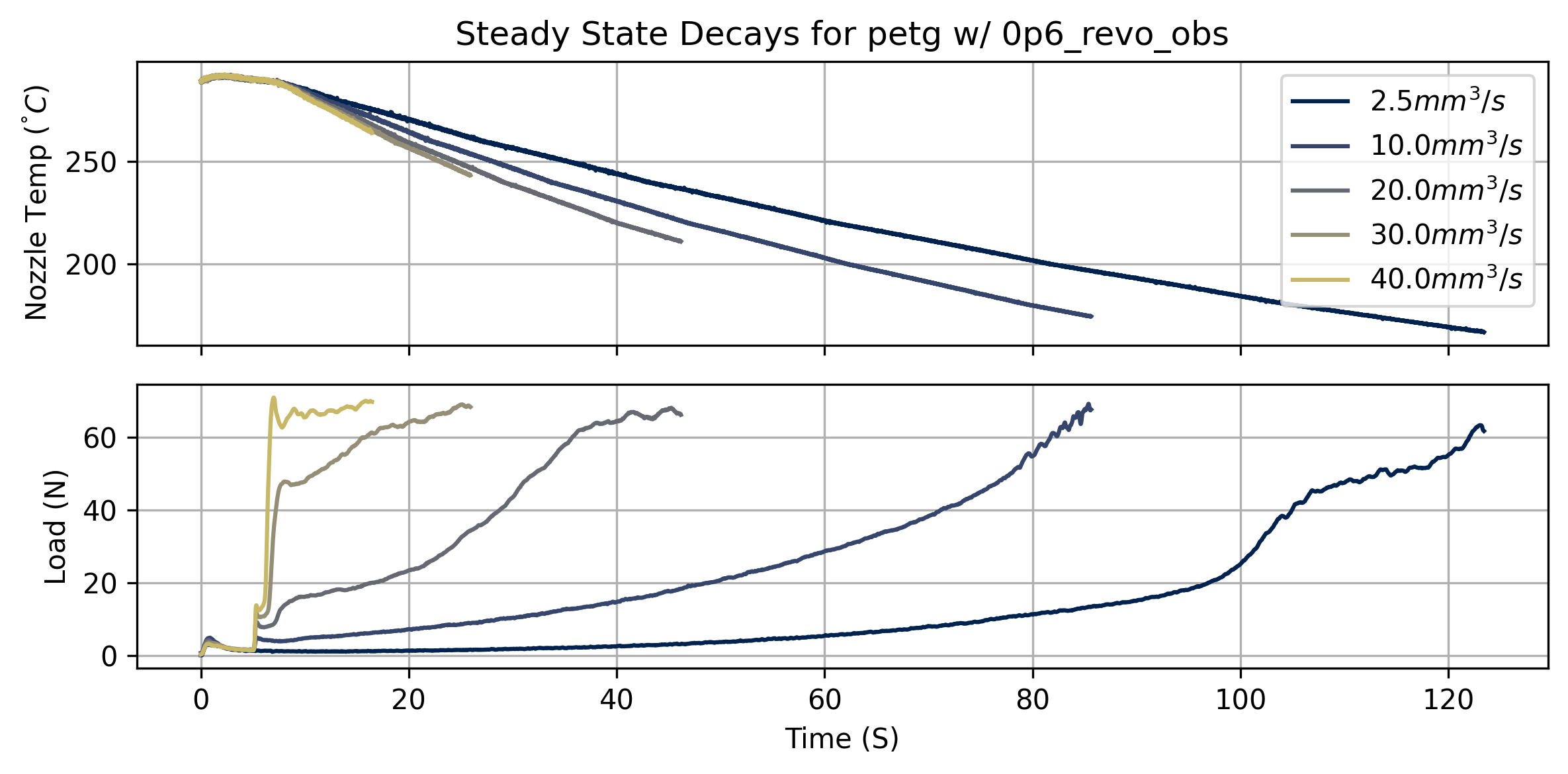

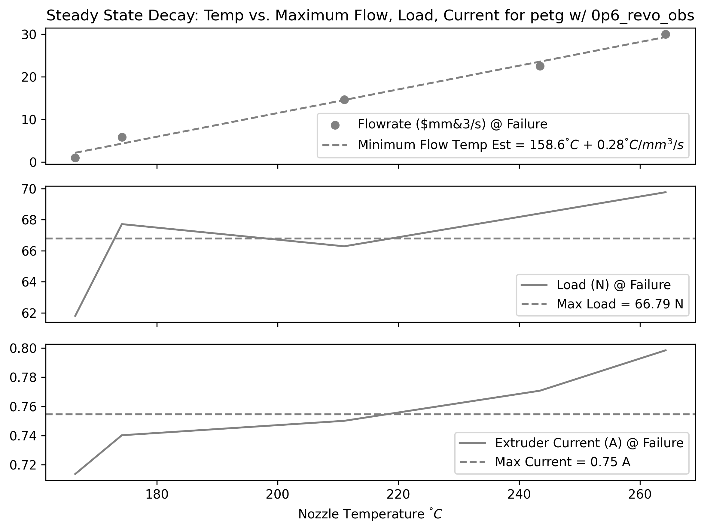
Listing 7.1: The test procedure that I use to generate melt flow steady state data.

Figure 7.6: Time series data from the steady-state decay test, generated with the routine described in Listing 7.1. Here, we heat the nozzle to it’s maximum temperature, and then flow filament at a set of constant rates while measuring all of our system states. The test stops when the extruder’s velocity controller fails to maintain the target rate, i.e. maximum extruder torque cannot sustain flow. Here we can see how pressure rises to some power as the temperature drops. We can also see that faster flowrates decay nozzle temperature faster, which we will use later on to characterize the materials’ volumetric heat capacity.

By measuring the temperature, loadcell, and motor current readings at the failure points for each test, we can extract simple estimates for the system’s maximum pressure and current across temperatures.

We can also fit a linear model for the minimum flow temperature across flowrates. The zero crossing of this linear fit is an estimate of the nozzle temperature where we might expect any flow to be possible; I call this the zero flow temp, or \(T_{min}\) - which we will use to normalize temperature ranges in some of the next steps’ fits.

Figure 7.7: Estimates for preliminary extruder limits, calculated from data in Figure 7.6.

In steadystate, our system is basically limited by the force we can exert on the filament, i.e. the pressure we can generate in the nozzle. In order to pick an operating region, we want to understand the relationship between nozzle temperature, pressure, and the resulting flowrate. So, some function:

\[ Q_{ss} = f_{ss}(F, T) \tag{7.1}\]

\(Q_{ss}\) is steady-state flowrate (\(mm^3/s\))
\(F\) is the loadcell reading (N)
- It is important to note that this is a pressure analog, not a direct pressure measurement. Reducing this measurement to a real nozzle pressure is presumably simple, but internal nozzle geometries vary by manufacturer, and an exact pressure measurement is not useful for our purposes of finding machine operating points (although it would be valuable if we wanted to deduce real viscosity measurements from our system).
\(T\) is the nozzle setpoint temperature (\(^\degree C\))
- Recall that this is not exactly related to the melt flow temperature, which may be substantially colder than the nozzle (especially at large flowrates, where the material does not dwell in the nozzle for long).

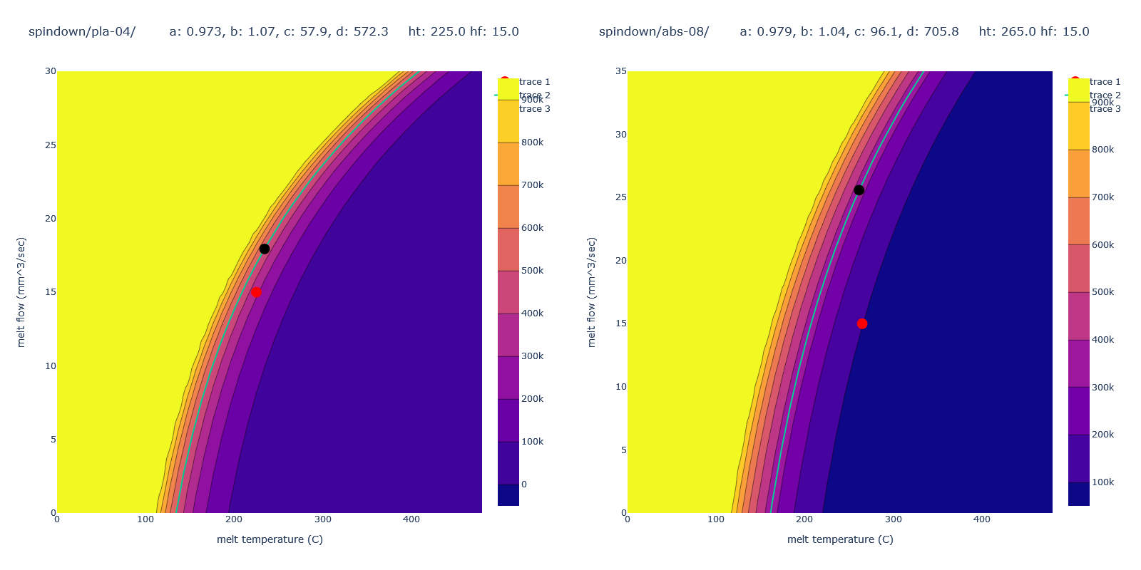
Before fitting across all temperatures, I fit a three-parameter isothermal model for steadystate flow across a selected range of temperatures. We generate a set of \(k_{off}, k_{lin}, k_{pow}\) for each temperature.

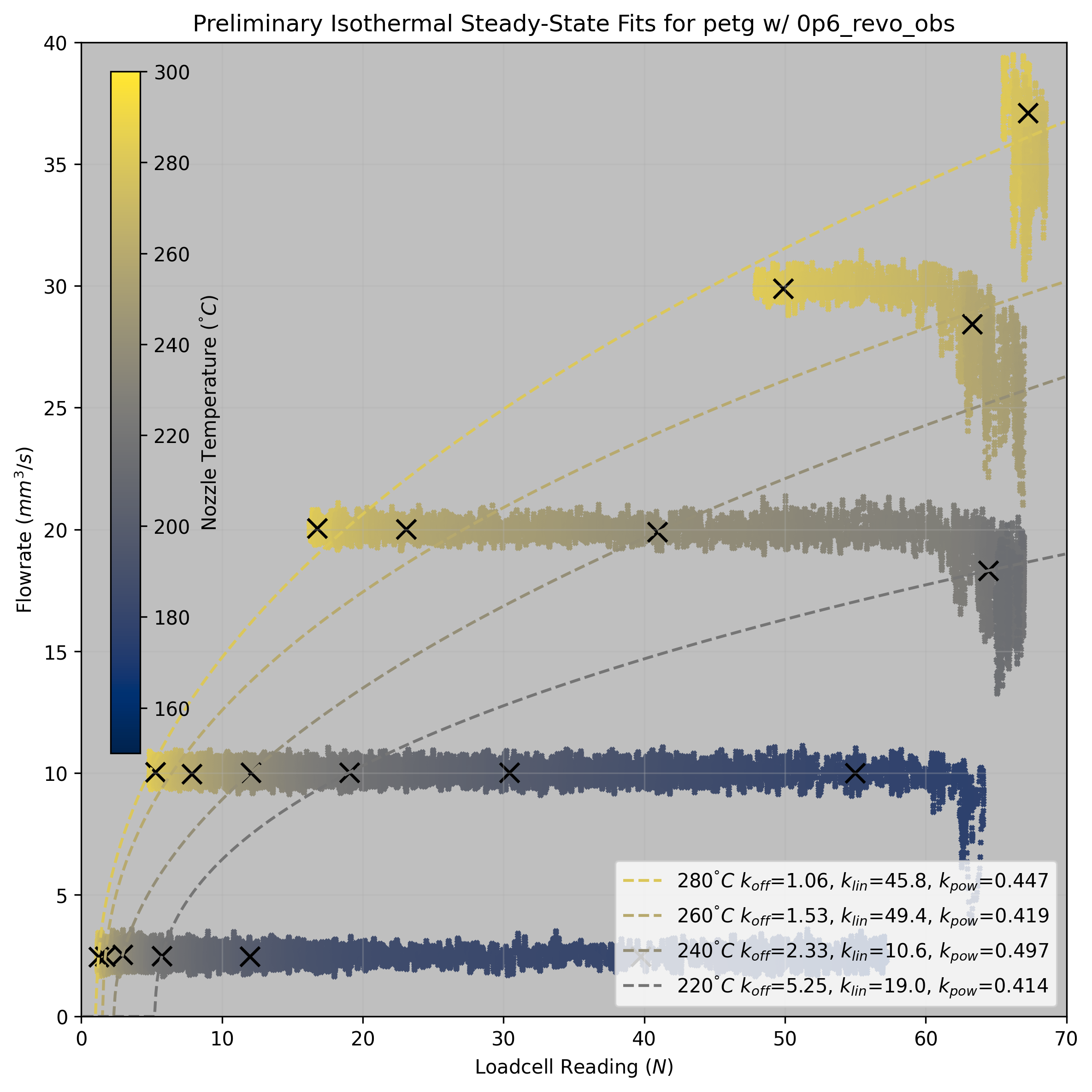
Figure 7.8: Test data from an experiment for steady-state flow data, which we fit to a function that estimates flow at a given loadcell reading, \(Q_{ss} = f(F) = ((F - k_{off}) \cdot k_{lin}) ^ {k_{pow}}\) - at this we fit unique parameters for each temperature, before fitting across all temperatures.

These preliminary fits are useful to get a sense of the system behaviour, but we really want to fit a function across any extrusion force and temperature. We can extend the isothermal model (Equation Equation 7.2) across temperatures by fitting an additional set of parameters that modify the first across temp.

\[ Q_{ss} = f(F) = ((F - k_{off}) \cdot k_{lin}) ^ {k_{pow}} \tag{7.2}\]

\[ \begin{aligned} Q_{ss} = f(F, T) = ((F - kt_{off}) \cdot kt_{lin}) ^ {kt_{pow}} \\ kt_{off} = ((T_{max} - T) \cdot a)^b + c \\ kt_{lin} = ((T - T_{min}) \cdot d)^e + f \\ kt_{pow} = g \end{aligned} \tag{7.3}\]

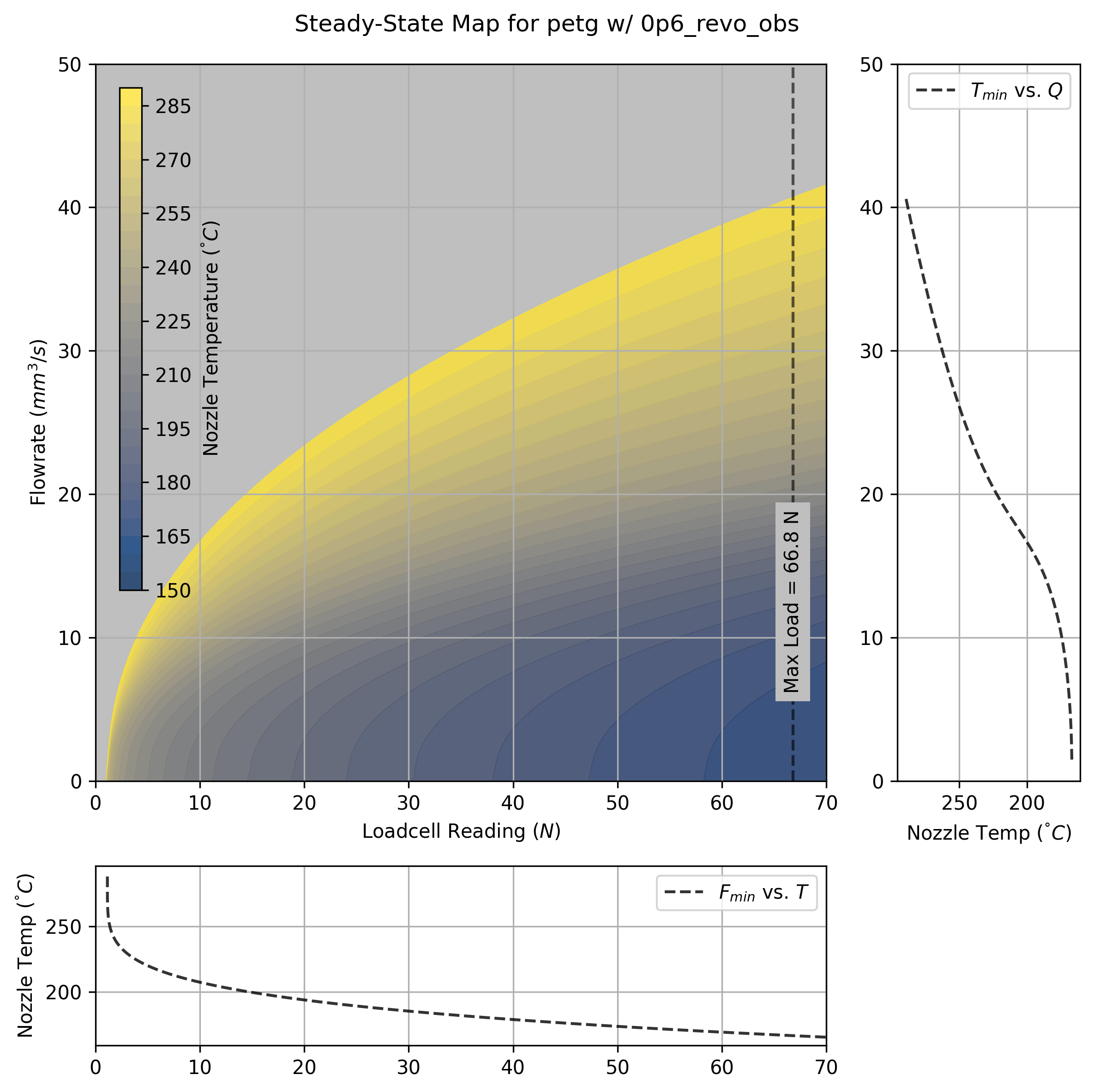
Figure 7.9: This contour plot predicts the steady-state extrusion rate (y) for any extrusion force (x) and nozzle temperature (z). The slice through maximum extruder load (at right) provides an operating boundary, and the slice through zero flow (bottom) shows us how much deadband pressure is needed before flow begins at each temperature.

The map is not exactly a physical model, but we can extract some useful information from it. Firstly, a slice through the maximum extruder load value sets a boundary for our dynamic operation, i.e. a maximum flowrate across a range of temperatures. We use this slice to set a boundary on our dynamic map in the next subsection (see Fig. Figure 7.11). A slice through zero flowrate shows us the deadband pressure across temperatures.

7.3.2.1 Implicit Thermodynamics in the Steady-State Model

The parameters for \(kt_{lin}\) and \(kt_{pow}\) are related to some physical phenomenology. The inverse of the power term tells us how quickly pressure increases with respect to flowrate, which we can understand physically as the coupling of the nozzle’s thermodynamics with the material’s viscosity across temperatures. Recall that at higher speeds, the melt flow does not reach the nozzle’s setpoint temperature (as it does not dwell for long enough to heat up) - this means that as flowrate increases, we have a compounding increase to the extruder load: first, we need more pressure to make more flow, and second, the decreased melt flow temperature increases the viscosity of the material, meaning we need more pressure again for the same flow.

As I will discuss later, the missing component of this model (and the one that would link our steady-state model with the dynamic model) is these thermodynamics: what is hidden to us (but could presumably be fit as a few hidden states) is the melt flow’s actual temperature, which is challenging to model because it is history dependent - that is, we would need to track the changing temperature of each segment of filament as it makes its way through the melt zone. This would involve fitting a more complete thermal model for the hotend itself (including i.e. thermal capacities and resistances for each of its components), and thermal resistance between the nozzle and filament (and conduction of the filament itself). We can easily generate enough data to build these models, and I expect it could be quickly developed by a heat transfer wizard. I am not one such wizard, and so I have quit this effort where it stands.

A final challenge with time-dependent thermal models is that they are maybe difficult to work with in the type of parallelized simulation / optimization routine that runs the printer in realtime, where accumulating states linearly through time imposes large performance hits (see Sec. Section 7.5).

7.3.2.2 Picking Parameters from Steady-State Maps Alone

In earlier work (Read et al. 2024), I showed that this steady-state model alone was enough to pick print parameters for many filaments, using a heuristic to find a zone within this fit that works across maps. For example I chose to operate the printer 80 \(^\degree C\) above the zero-flow temperature, and at 75% of the maximum extruder load.

This alone was sufficient to build viable parameters for printing, but was clearly missing the dynamics required to have the machine start and stop tracks properly. In the next section, we will look at how to address this component of the system.

Figure 7.10: These “3DBenchys”¹(CreativeTools, n.d.) were printed using a classical workflow, but with parameters selected from steady-state maps similar to those fit in this work Section 7.3.2.

7.3.3 Isothermal Dynamics for Pressure, Flow, and Compression

So, the steadystate model helps us to set operating boundaries for our machine, but it does not properly model operation of the system during short time intervals, and with rapidly changing inputs to target flowrate as is common under real printing conditions.

Recall in Fig. ?fig-extrusion-explainer that the filament between the drive gears and nozzle tip acts as a spring: this means that we need to anticipate increases to extrusion rate by preloading this spring, and anticipate reductions to extrusion rate by unloading the spring. This is handled approximately in state of the art printer firmwares approach called linear advance (P. Research, n.d.). However - this is a firmware setting. Not all controllers allow this to be modified without re-compiling a firmware, and those that do allow this need the slicer to tell them where to set it. Filament compressibility is not just dependent on the filament (whose stiffnesses vary wildly), but on the printer design (some have better extruder designs than others) and the flow temperature (warmer melts are more compressible).

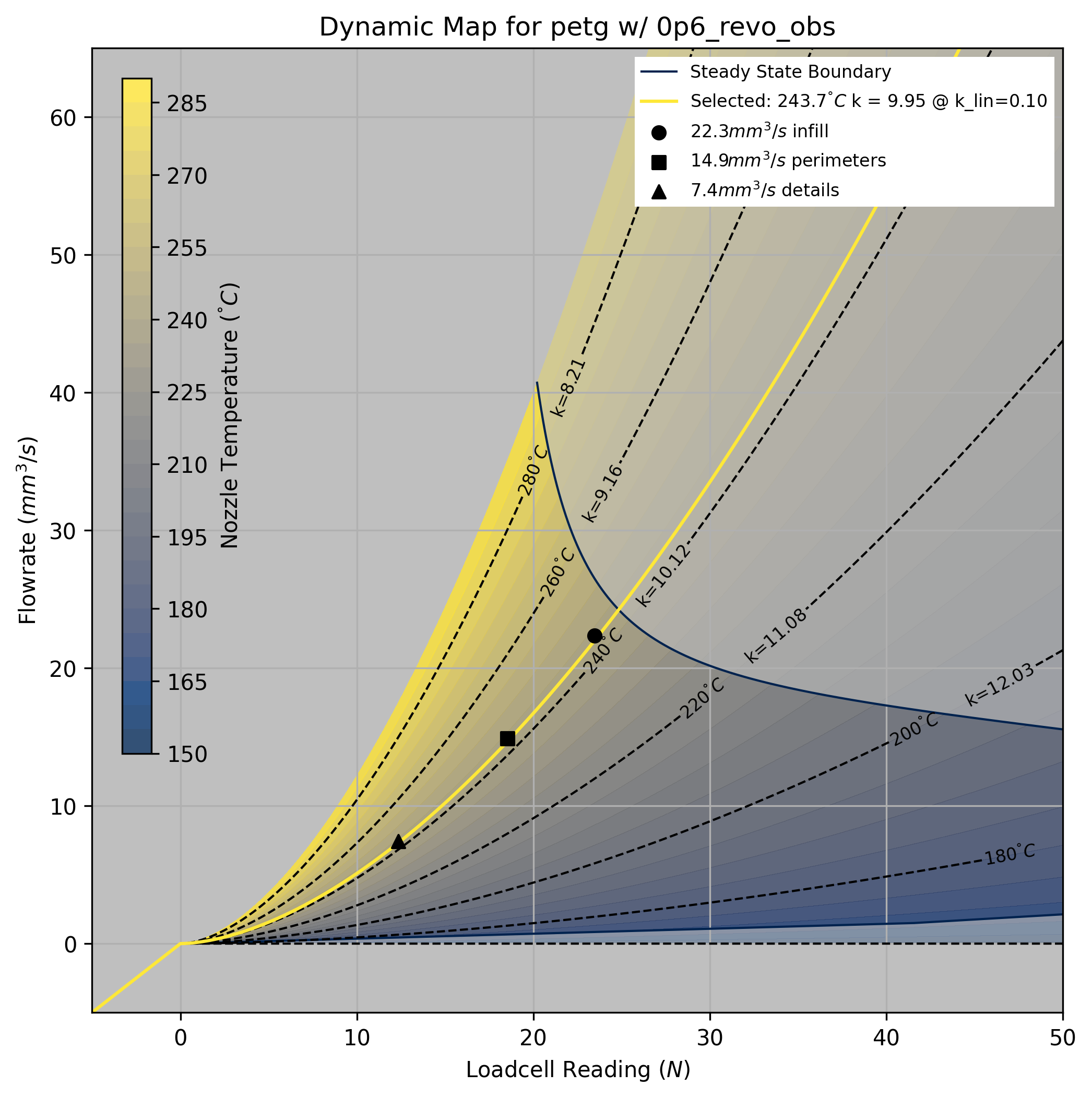
Figure 7.11: This is the pressure (horizontal axis) to flow (vertical axis) across temperatures (colormap) for PETG, with a 0.6mm nozzle. The yellow line calls out a temperature that was selected where the flow’s linear term is `0.1` - a model heuristic that I discuss in Section 7.4.3.1, and the marked flowrates are selected as using proportions the maximum load at this temperature.

For compressibility, we fit a compression parameter \(k_{sq}\) to the filament, which estimates how much nozzle load is generated for each cubic millimeter of filament that is compressed between the extruder motor and the nozzle tip. This is effectively a springrate (units are \(N/mm^3\)): with softer filaments, we need to spin up our extruder motor further in advance of our desired outflow, whereas stiffer filaments are more direct. As we would expect, melt flows at higher temperatures are softer (less springrate) than those at cold temperatures.

The pressure to flow relationship is also different on these shorter time scales; here the phenomenology is more what we would expect from a non-newtonian fluid. Recall that for an isothermal flow of a newtonian fluid, we would expect pressure and flow to have a linear relationship. In these models, we see a power relationship, i.e. flows are typically described by some function Equation 7.4, with a linear term \(a\) and power term \(b\).

\[ Q = (Fa)^b \tag{7.4}\]

In our steady-state model above, as pressure increases, steadystate flow increases but at a decaying rate - i.e. for every additional N of load, we get less return on flow (\(b < 1.0\)). However, on shorter time-scales, this is reversed: flow increases at an increasing rate for every additional N of load (\(b > 1.0\)). As already discussed, the decaying exponent in steadystate can be understood as the melt flow’s temperature dropping at larger rates (thus increasing its viscosity). On short time scales, we see polymer shear thinning[^SHEAR_THINNING], a phenomenon observed in non-newtonian fluids where increases to pressure (… shear) drop the flow’s viscosity.

7.3.3.1 Fitting Dynamic Models

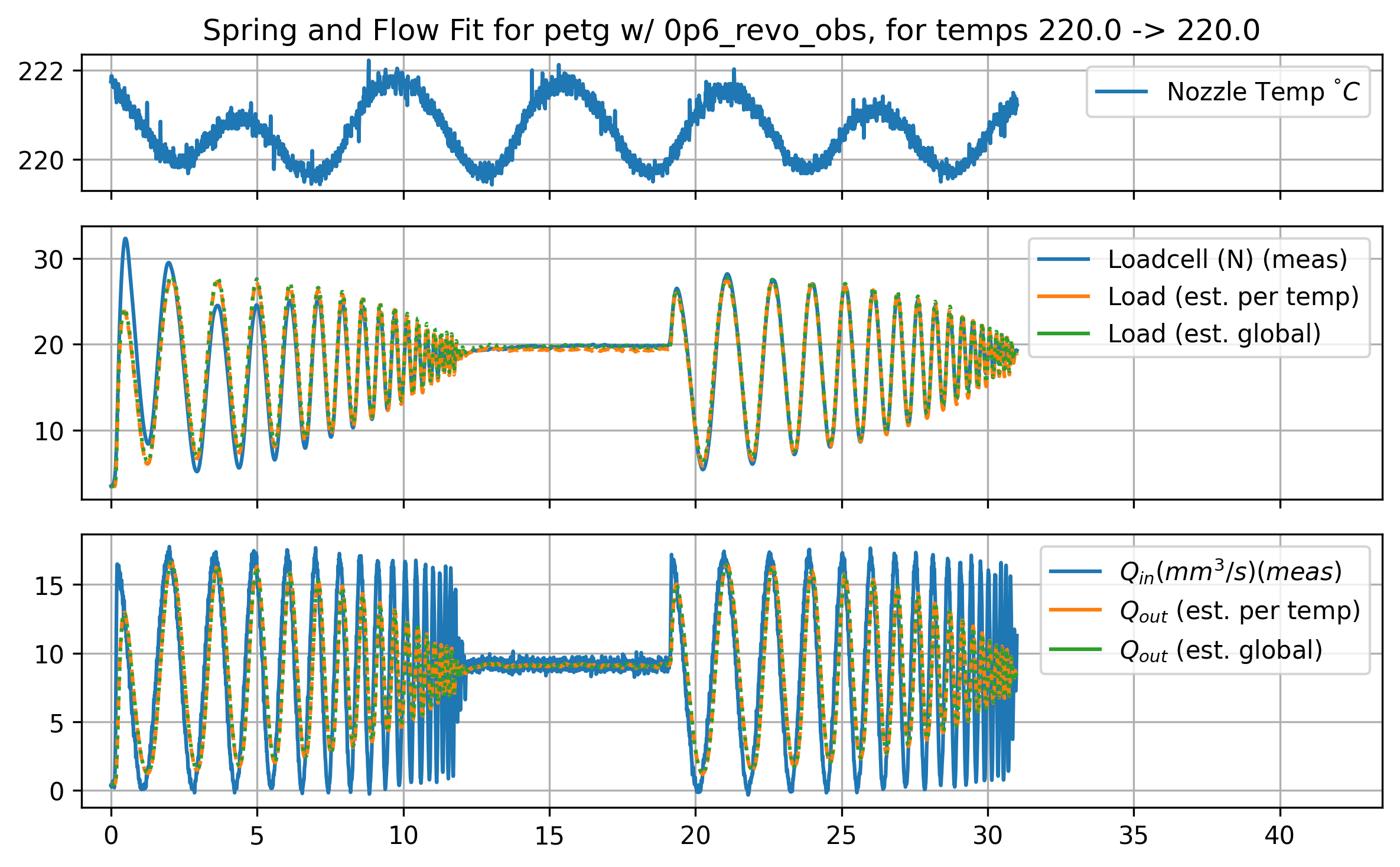
For dynamics we naturally want to fit some set of ODEs that will predict time-series behaviour of the system. Those are below in Equation Equation 7.5

\[ \begin{aligned} Q_{out} = (Fk_{lin})^{k_{pow}} \\ \dot{F} = (Q_{in} - Q_{out})k_{sq} \end{aligned} \tag{7.5}\]

The driving input to this set of ODEs’ is the extruder velocity (inflow, \(Q_{in} (mm^3/s)\)) and output is the flowrate from the nozzle tip (outflow, \(Q_{out}\)), with an internal (compression) state (our loadcell reading) \(F (N)\) - this is scaled by the springrate \(k_{sq}\)

In prior work, I fit the springrate using computer vision, but I have found that we can simplify this step by adjusting the parameters’ of those ODEs so that our time-series data for extruder load aligns with the models’ simulation, i.e. we fit to the internal state rather than the final output. This greatly simplifies the data gathering routine, allows us to extend modeling across all data gathered from the machine, and fit on higher frequency data (camera frames are gathered around ~ 30Hz, but loadcell data arrives at ~1kHz).

The appropriate data to gather for a starting fit is a simple chirp signal sent into our extruder’s velocity controller. A chirp works well because it causes our model to fit the dynamic state (compression) across a range of frequencies, whereas the pressure relationship must fit consistently across the whole of the chirp.

Figure 7.12: This plot shows time-series data from one of the chirp tests used to fit parameters for the flow dynamics ODEs in Eqn. Equation 7.5.

7.3.3.2 Dynamics Across Temperatures

Parameters for the flow system vary across temperatures: warmer flows have smaller springrates (are more compressible), and tend to have more linear pressure-to-flow relationships. This makes intuitive sense: hot things are less stiff, and more molten (less viscous) flows act more like newtonian fluids: with less viscosity overall, pressures at the same flowrates are lower, meaning we have less shear and less nonlinear shear thinning.

While it would be possible to simply use the parameters we find at the temperature we choose to operate in, we can also fit a relationship between these parameters and the nozzle temperature. This helps us later to pick an exact temperature to operate with, and prevents us from having to fit parameters for any temperature we would like to fit.

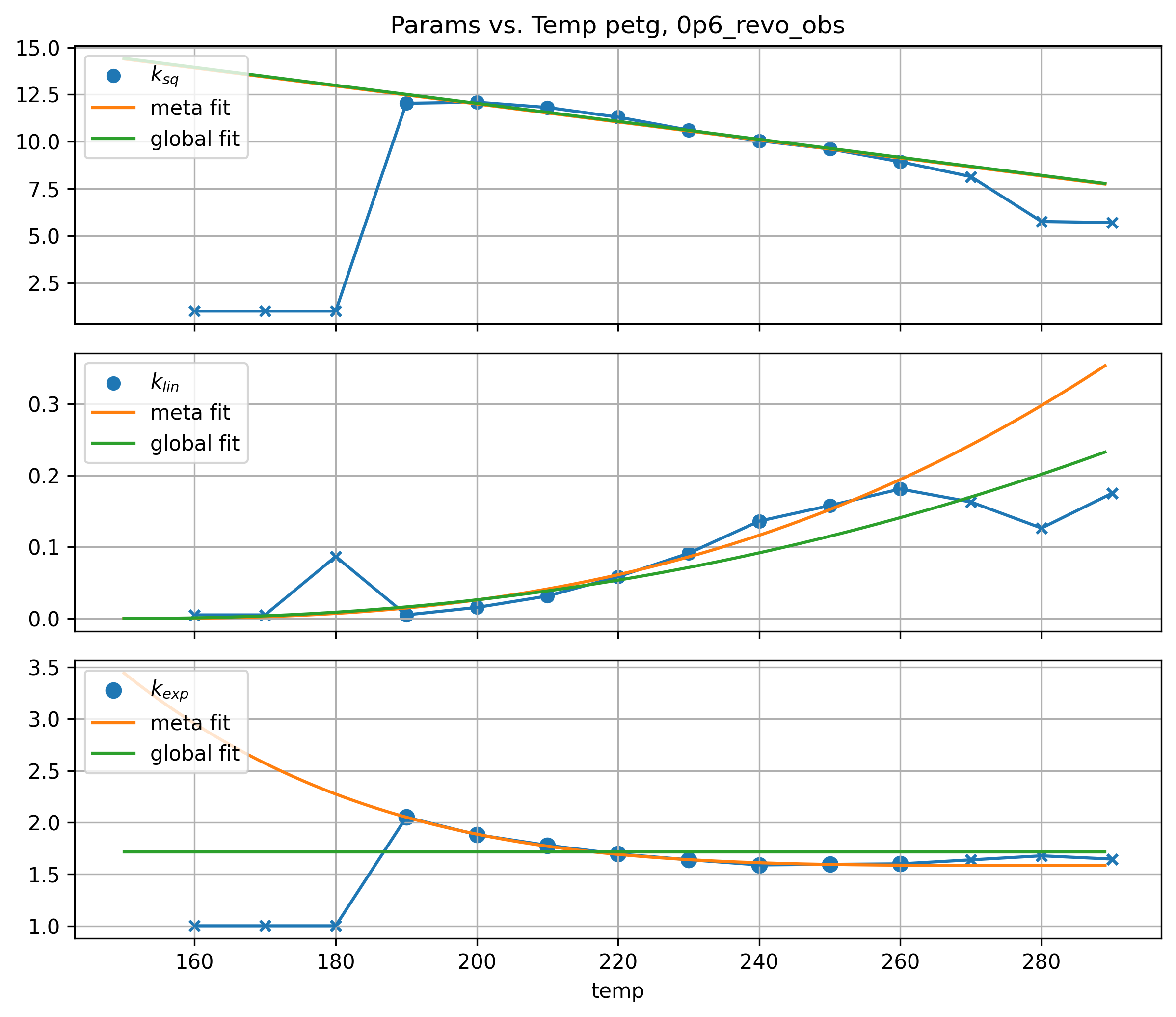
After gathering datasets for a few filaments, I looked at paramters across temperatures and saw some simple relationships: the springrate is linear (decreasing) with temperature, the linear term in the pressure-to-flow relationship tends to increase exponentially with temperature, and the exponential term of the pressure-to-flow relationship tends to decay exponentially with temperature (approaching 1.0).

As we did with the steadystate model, here we fit some additional terms that modify our underling parameters across temperature.

\[ \begin{aligned} kt_{sq} = (T_{max} - T) \cdot a + b \\ kt_{lin} = ((T - T_{min}) \cdot c) ^ d + e \\ kt_{pow} = ((T_max - T) \cdot f) ^ g + h \\ \end{aligned} \tag{7.6}\]

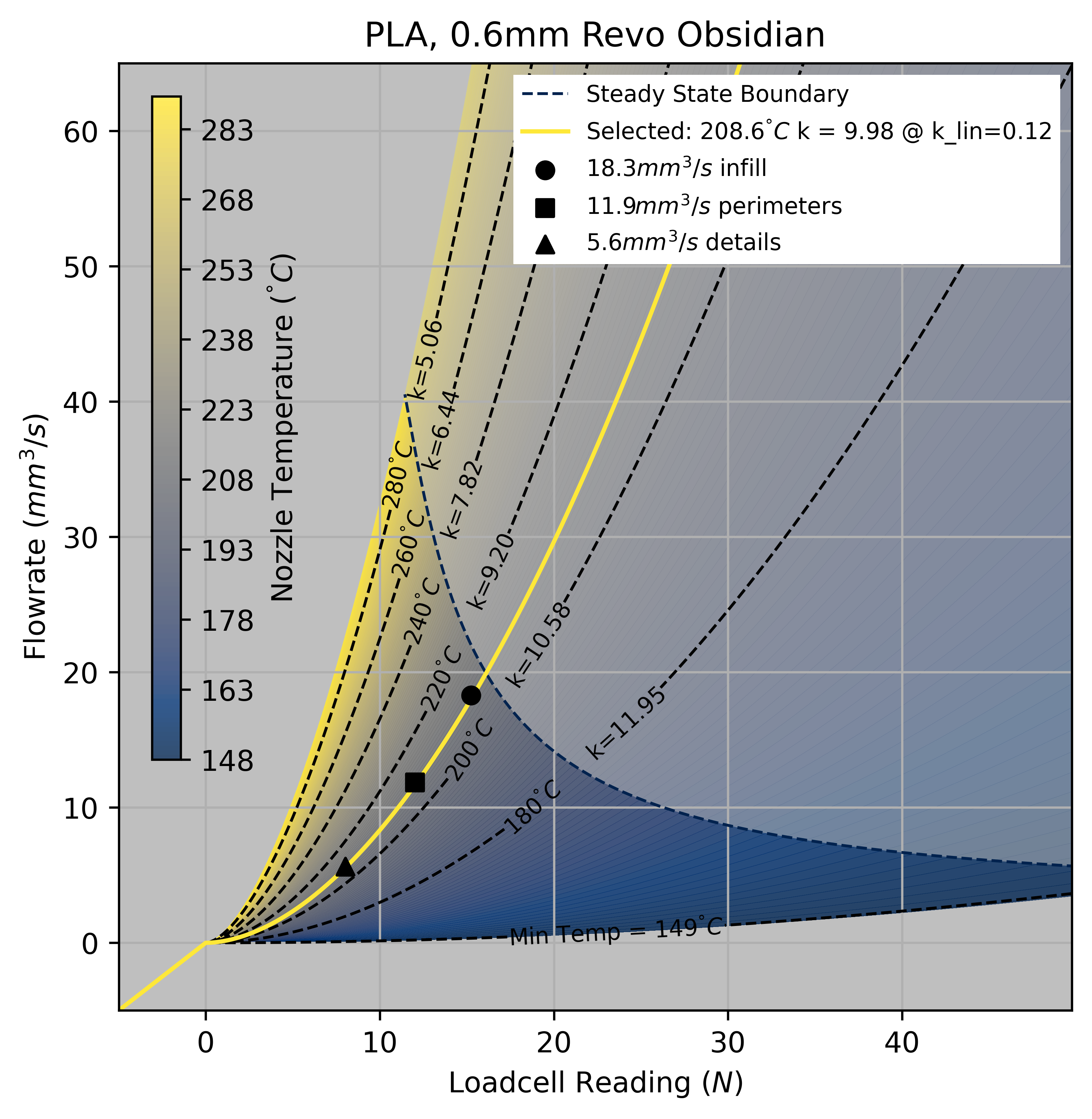
Figure 7.13: Here we see isothermal flow parameters across a range of temperatures, and fits for these parameters via two strategies: a ‘meta fit’ via tuning \(a...h\) against previously fit parameters directly, and a ‘global fit’ where we tune the parameters end-to-end. While the meta fit predicts per-temperature parameters more successfully, the global fit is preferred since it’s error map is more closely aligned against the actual data we want to predict.

Putting this together with the steady-state boundaries discussed above, we can produce operating maps like those below that display dynamic characteristics across temperatures, including springrates (marked on temperature contours) and boundaries. In the next section Section 7.4, I will explain how we choose an operating temperature (and set of flowrates) out of this region.

Figure 7.14: Here we show dynamics maps for PETG and PLA, both on the same extruder and nozzle. TODO: add PLA… yada yada

7.3.4 Interploating Between Steady-State and Dynamics Models

Real world operation of the machine is not isothermal like the dynamic model (NOTE: should rename that to the isothermal model, dadoi). In practice, the internal temperature of the melt flow (which is impossible to measure directly) is not exactly matched to the nozzle temperature.

This is where the modelling becomes tricky. But there is some hope. If we compare our steady-state and isothermal models, we can see that each returns a nozzle temperature for any point in the (pressure, flowrate) space.

Figure 7.15: The isothermal model for flow in PETG (left), and the steady-state model (right).

If we assume that our isothermal model works, we can measure the actual melt flow temperature for each point in our steady-state map. That is, for each point (pres, flow) in the steady-state map (at a given nozzle temperature), we can find the same point in the isothermal map (at a different temperature). This results in a third map that renders \(\Delta T\) for any flowrate and nozzle temperature.

Steady State to Isothermal Interpolation (3D)

Figure 7.16: Interpolating between Steady-State and Isothermal Flow Maps helps to understand the non-isothermal behaviour of the flow: for any average velocity of the flow in the melt zone (aka the dwell time), we can estimate the melt flow’s internal temperature, and use that to determine the true flow parameters at that operating point.

We can then reason that the average speed of the filament in the melt zone, together with the nozzle temperature, will tell us what the melt flow’s actual average temperature is. This approximation comes short of a complete thermal simulation of each component of the flow (which would be computationally expensive to compute), but (?) works well to simulate the dynamics.

7.3.5 Extruder Motor Dynamics

Besides all of these melt flow dynamics, our extruder motor is also subject to the physics we discussed in Section Section 6.1. When we analyse printing data later, we will see that overall print speed is often limited by the extruder motor’s ability to rapidly compress and decompress filament as the machine corners. It must also provide enough torque to sustain nozzle pressure during steady motion, indeed this section opened up by finding maximum flowrates that are limited by our ability to generate extruder pressure.

For a refresher on motors: we have a direct relationship between stator current and torque produced by the motor. This means that motor torque is limited by current saturation, which can come from either the driver circuitry’s power limits or the motor’s own thermal limits. Most 3D Printer designs favor small extruder motors that are limited to about 0.5 amps of continuous drive current.

Current in a motor cannot change instantaneously (due to coil inductance, this results in a jerk limit), and current generation is further limited at high speeds due to stator reluctance and back-emf voltage. Again, see Section Section 6.1 for more detail on the topic, we get into it bigtime.

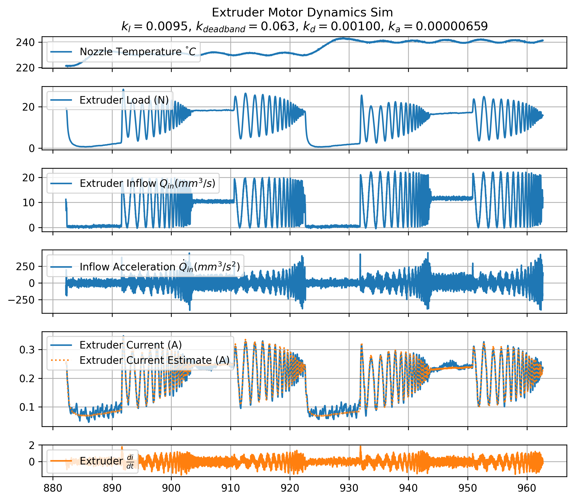
Motor dynamics are typically coupled into motion systems that have fixed mass and damping (except for those with nonlinear kinematics). In the extruder system, we need to add a parameter for the amount of current required to generate pressure in the nozzle. This means that in the case of the extruder, we need to build a model that predicts motor current as a function of the motor’s speed (a damping term), acceleration (inertial), and an additional fit for the load to current relationship. This is below in Equation Equation 7.7.

def extr_qcur_estimator(params, load, rate, accl):
    kl, kl_deadband, kd, ka = params 
    qcur = np.where(load > 0.0, (load * kl + kl_deadband), 0.0) + rate * kd + accl * ka 
    return qcur

\[ \begin{aligned} I_{extr} = Lk_l + k_{deadband} + Q_{in}k_d + \dot{Q}_{in}k_a \\ k_l = \text{Linear Load Factor} \ (A/N) \\ k_{deadband} = \text{Load Offset} \ (N) \\ k_{d} = \text{Damping} \ (A/mm^3/s) \\ k_{a} = \text{Inertial} \ (A/mm^3/s^2) \end{aligned} \tag{7.7}\]

The damping and inertial terms are fit again in terms of the inflow - i.e. the flowrate past the extruder’s drive gears, which is exactly proportional to the extruder motor velocity (with some scalar).

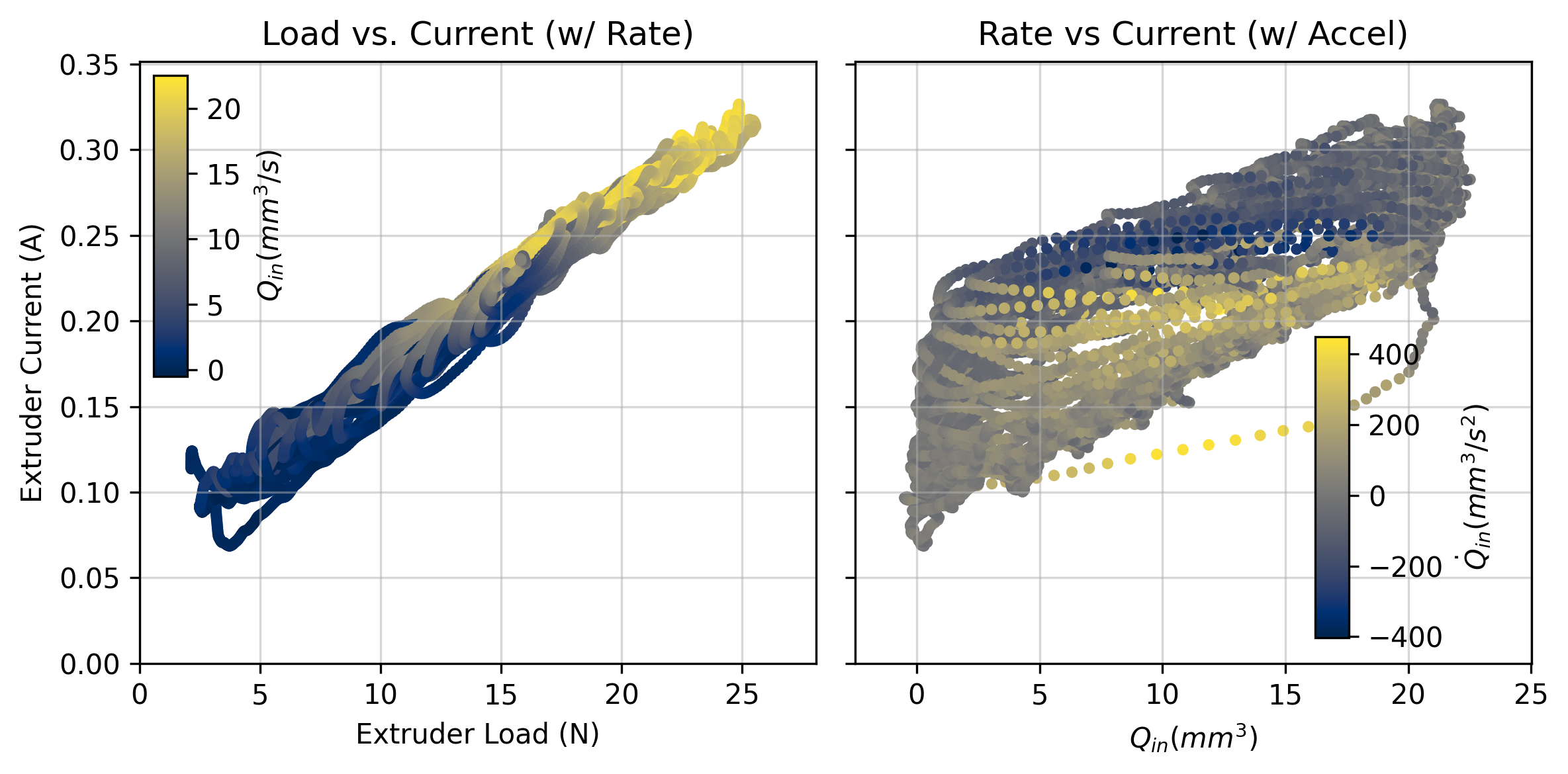
Figure 7.17: Here I plot extruder current (y axis, both plots) against the loadcell reading (x-axis, left plot), rate (colormap, left plot, and x-axis right plot) and acceleration (colormap, right plot). A linear combination of these three states predicts the extruder current well: load is the dominant factor, rate contributes significantly as well. While acceleration’s contribution is small, it is important to model because dynamic operation often requires rapid changes in extruder velocity.

Finding the parameters for this model is simple with time series data. We typically see that our current requirement is dominated by the extruder load, with a smaller damping parameter and even smaller acceleration parameter. Even though it looks small, the acceleration parameter often becomes the critical limit during dynamic moves where optimal inflow acceleration requests can exceed \(10000mm^3/s^2\). Parameters from an example fit are called out in Figure Figure 7.18 below, where I compare time-series measurements (in blue) to the model’s estimates (in orange).

Figure 7.18: Extruder motor parameters for current estimates are fit using the motor modeling routined discussed in Section Section 6.1. To fit the parameters that link the motor model into the extruder model, we use dynamic data from the flow chirp time-series, which are plotted here. Parameter fits from Equation Equation 7.7 are called out, and the estimated current is compared to the measurement.

7.3.6 Die Swell

TODO: we have some data for this… not sure if it will make it in. Maybe 1day for modeling, but current plans don’t anticipate using it at all. Though it might be interesting to show. Will write it up at that time if it seems useful. It is maybe kritical to show because in some systems we have lots and lots of extruder current but our actual maximum rate should properly be limited not by the max force, but by die swell…

It’s fusili Jerry ! FIG: radiator pasta: CAP: The radiator pasta, via extrusion. The curl emerges from die swell: radiator fins extrude at a higher pressure, and so become larger than the flat section after extrusion, which causes the radiator to wrap.

Curious ragu enthusiasts among us may have wondered how radiator pastas get their wonderful, sauce-hugging shape. The answer is die swell, a phenomenon where flows that are extruded at high pressures bounce back to become larger than their die’s orifice once leaving the extruder.

In pasta shape development, this is a wonderful trick that lets us make non-euclidean pasta shapes. In printing, die swell is bad: it means that the tracks we print are not the width we expect, and as they cool they contain residual stresses.

Die swell occurs mostly when we extrude polymers when they’re not completely liquefied (which they never are?) - i.e. one way to think about it is as the filament’s memory - when we extrude filament near maximum pressure (at low temperatures), it returns to about the same width as it was when it was solid filament - i.e. 1.75mm in our case.

I endeavoured to measure die swell with the small thermal camera attached to the rheo printer’s extruder, since the signal is quite useful not only for avoiding die swell itself, but for measuring which of our viable extrusion temperatures and rates will make for good print parameters. The camera is extremely low resolution, but (because the melt flow is obviously hotter than the background), it it relatively easy to pick out edges.

FIG: thermal camera frame, with width measurement taken from some slice?

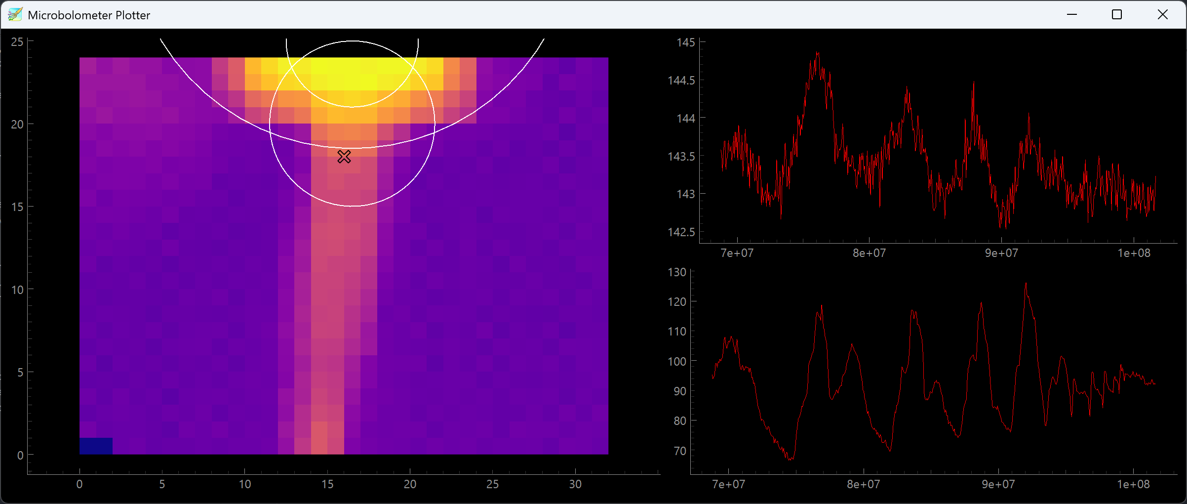
I use an approach known as “sub-pixel” sampling: TBD, WRITE UP WHEN DONE… yada yada, discussion on how it relates to pressure, temp, and what it tells us.

7.3.7 Filament Volumetric Heat Capacity

While it is difficult to develop a complete thermal model of our filament, we can at least estimate its volumetric heat capacity \((J/mm^3)\) - this value will be useful when we get to layer cooling time estimates (Section Section 7.4.3.2), and could be used in the future for predictive heating controllers / to connect our steady-state model and dynamics model.

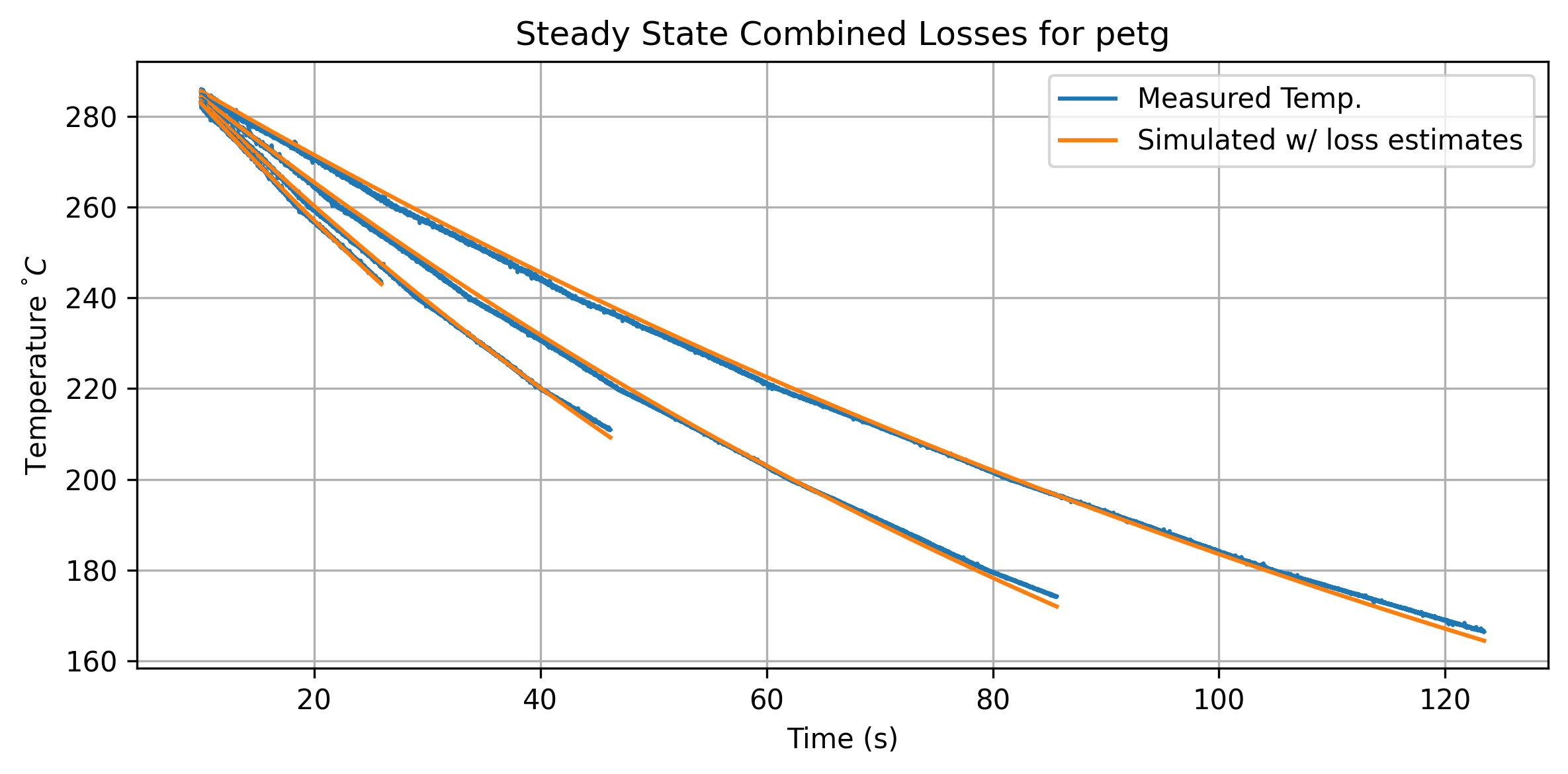
During our steady state tests, nozzle temperature decays due to losses into ambient environment and loss into the filament flow.

\[ \begin{aligned} \frac{dT}{dt} = (T_{ambient} - T) k_{loss} + (T_{ambient} - T) k_{flow}{Q} \end{aligned} \]

Temperature loss to ambient \(k_{loss}\) is a rate in units \(\frac{C/s}{\Delta T}\)
Temperature loss to flow \(k_{flow}\) is a rate in units \(\frac{C/s \cdot (mm^3/s)}{\Delta T}\)

The \(\Delta T\) we use for each of these losses is from ambient temp \(T_{ambient}\) to the nozzle temperature: making the assumption that filament flow heats from ambient up to the nozzle temperature before exiting the nozzle. To fit, we first estimate the total loss across each flowrate, as in Figure Figure 7.19.

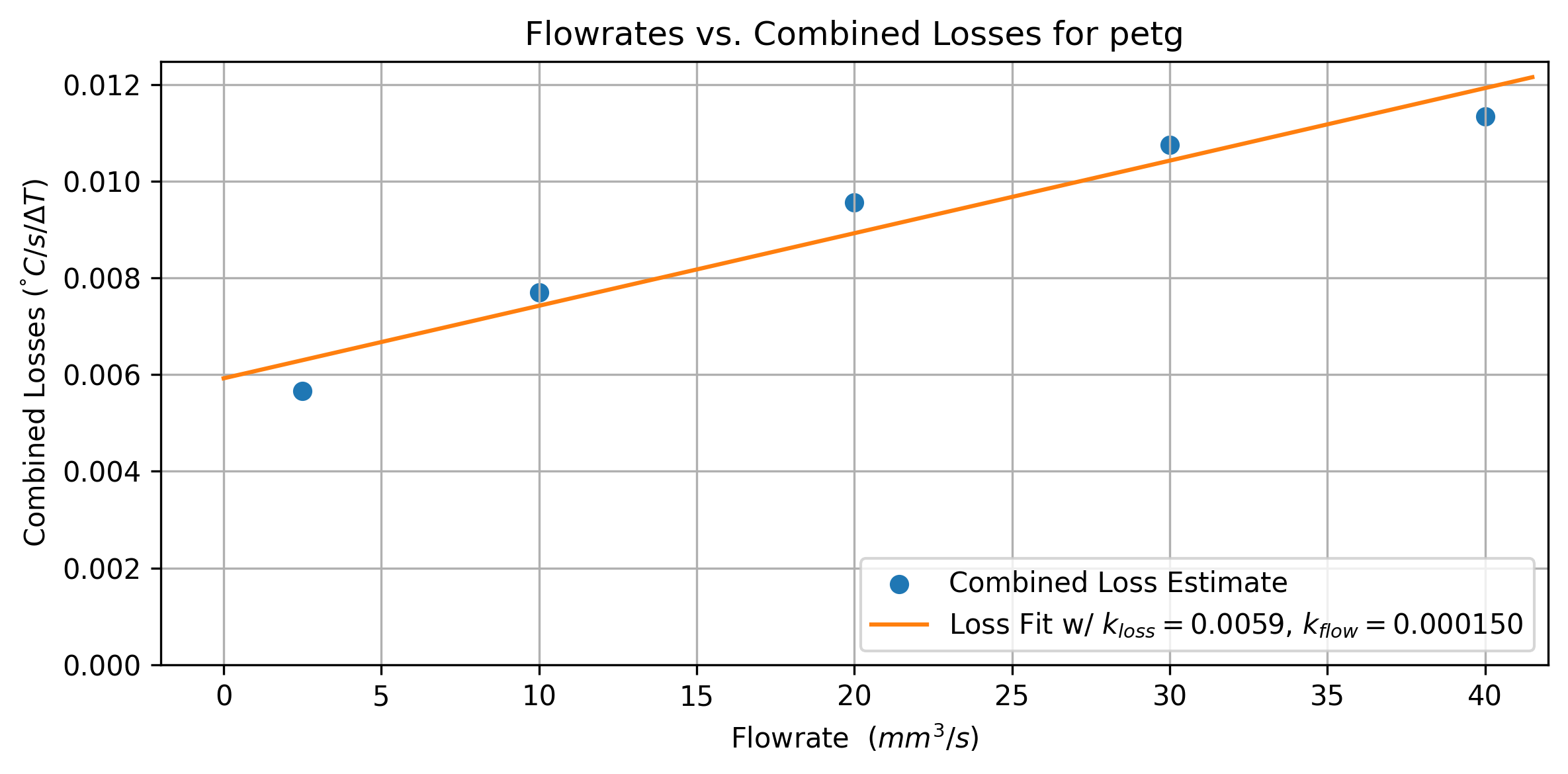Figure 7.19: This is the same data presented in Figure Figure 7.6, now overlaid with simulations using a combined loss.

Here we plot combined loss across rates, and our estimate for independent ambient loss and flowrate-dependent loss paramters. {#fig-extr-model-ss-loss-per-rate}

These losses are not yet power measurements. To back out a heat capacity, we need to measure the watts required to move the nozzle temperature. For this, we can fit an additional parameter that is active when the nozzle is warming up.

\[ \begin{aligned} \frac{dT}{dt} = k_{in}W_{in} + (T_{ambient} - T) k_{loss} \end{aligned} \]

\(k_{in}\) in units \(\frac{C/s}{W}\)
\(k_{loss}\) (from our prior fit) in units \(\frac{C/s}{\Delta T}\)

We can easily measure the power into the nozzle \(W_{in}\) by measuring our heater’s resistance and the controller’s supply voltage.

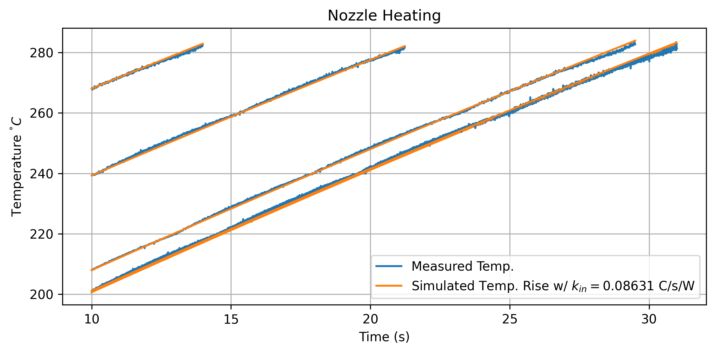It is easy to measure power delivery into the nozzle. We can use this constraint to fit an estimate for a conversion between the rate of temperature change and the heat energy flow into (and out of) the nozzle. {#fig-extr-model-temp-rise}

We can now combine our measurements to produce an estimate for the filament’s heat capacity. If we do a little bit of units analysis, we can see that the volumetric heat capacity is equal to \(k_{flow} / k_{in}\) -

\[ \begin{aligned} C_v = k_{flow} (\frac{C/s \cdot (mm^3/s)}{\Delta T}) / k_{in} (\frac{C/s}{W}) \\ \frac{C/s \cdot (mm^3/s)}{\Delta T} \cdot \frac{J/s}{C/s} \\ \frac{(mm^3/s) \cdot J/s}{\Delta T} \\ \frac{J\cdot mm^3}{\Delta T} \end{aligned} \]

Mostly we measure specific heat capacity of materials (i.e. \(J/kg\)), but in our case volumetric is more useful - and we anyways don’t have a measurement for material density (although it is easy enough to make). To compare our measurements against available data, I have compiled the table below Table 7.1.

Table 7.1: This table compares measurements for volumetric heat capacity in this work (left column) vs. values available online. It also tabulates reference values for density and thermal conductivity.

Material	\(C_{meas}\)	\(C_{ref}\)
PETG	1.7	1.6 (?)
PLA	1.5	1.7 (?)
Nylon
NuTan		N/A
PETG-CF		N/A
HTPLA-CF		N/A
PCABS-GF		N/A
Alu Fill		N/A
Wood Fill		N/A

Our measurements are not incredibly precise, but do put us in a reasonable ballpark for the real physical value. Polymer heat capacity is anyways nonlinear in practice (CITE?), with i.e. different phases of each polymer having different heat-carrying capabilities (not to mention density changes). For our purposes, an estimate is good enough, and also goes to show the types of data that can (surprisingly) be backed out of simple tests on instrumented machines.

7.3.8 About Non Isothermal Melt Flows

Subtitle: everything missing from this modeling effort… i.e. future work.

I do want to look at… steps towards better thermodynamics models in filament flow. Includes: non-isothermal, filament thermal resistance (PETG, PETG-CF…), and actual cooling time estimates (from bolo)

I want to discuss briefly an aspect of the melt flows that I was unable to completely figure out, which is the thermal modeling across longer time dynamics.

Everything I have discussed so far models isothermal conditions, where we take for granted that the polymer melt in the hotend is roughly the same temperature all the time. This is not the case at sustained high speeds, which limits our operation to regimes that are isothermal in steady state (as discussed).

To demonstrate, let’s look at a pressure (and die swell ?) trace from a period of sustained flow near the steady-state limit.

FIG: trace with some kickoff !

Despite our inputs remaining steady, pressure spikes at (?) seconds into the run. This takes place roughly when the cold filament bottoms out in the melt zone… i.e. when the fresh chunk of filament reaches the nozzle tip.

Yada yada, much more pressure (none of the filament is molten), much bigger springrate, IDK how to model this, velocity averages can help, etc.

To show how nozzle thermodynamics affects steady state flowrates, we can look at data for two systems that are identical (PLA, 0.6mm Nozzle) except that one nozzle is (STEEL?) and the other is (COPPER?), meaning the latter conducts heat from the cartridge to the filament at a higher rate (FIGURE: looking at nozzle thermodynamics?).

Comparing flow models from high- and low-conductivity nozzles.

Figure 7.20: Caption !

The copper nozzle shows higher steady-state flowrates overall, but a smaller slope… yada yada.

NOTE: these thermal models are incomplete… and mix thermal capacities, resistances, … to properly understand these models, we would want to add a test thermistor in the nozzle, and use chirp data…

MAYBE INCLUDE: thermal models that estimate tau - but maybe not worth discussion? Though they can be used to tune PIDs.

TODO: compare here… steady-state boundaries vs. dynamics models for PETG, PETG+CF: we should see that steadystate models more of the conductivity of the filament, whereas in the isothermal model this difference is less pronounced… need to actually get those figures to compare.

DISCUSS: hotter, slower makes for better layer adhesion as noted by… JON (cite)… we should be able to operate on a pareto frontier… and even more-better would be to ramp rates depending on layer size; research on these fronts is active in the FFF community (also largely outside of academia…),

7.3.9 Other Modeling Candidates

tried neural nets, they can fit well but work poorly when we leave the boundary of data previously collected

Related to overall compute performance, we need to learn what fidelity of model is required for our real-time optimization task. Candidates include classical models (that are hard to build but easier to fit, and faster to run), various flavours of neural network (which are easier to train but slower and less relate-able to underlying physics), and even particle simulations.

Here I show the littany of of model gathering and fitting techniques that I tested as I developed the Rheo-Printer, as well as a shared functional representation for the differentiable simulation (simple integrators) and optimizer. I also evaluated two solver architectures, and two different approaches for deploying synchronized motion segments.

7.4 High Level Planning with Models

The models I have developed for melt flows work well to characterize the basic phenomenology of the system, but there are a few aspects of FFF printing that they can’t directly tell us about, and that happen at time scales longer than anything the solver will look at. As ever, there is still room for heuristics.

However, rather than being pure heuristics, these are model based, so i.e. we can tune heuristics through our models: this lets us develop our heuristics in a way that they are automatically broadcast across materials. To apply these heuristics to print jobs, I build a preprocessor with three inputs: the print geometry, our models, and this (small) set of heuristics / hand-tuneable parameters (see Figure 7.4). This preprocessor is basically where I stick all of the things that I think off-the-shelf slicers should incorporate.

This section may seem a little bit strange, because it at times will look relatievely measured and scientific, and at times I will basically throw my hands up and say “we use x value for this, because it works.” This is kind of the point: we are blending models-based operation with hand-wavey heuristics. We do this because it works and reaching further for more advanced models and optimizers would not be worth our time².

7.4.1 First Layer Speed

FFF veterans know well that the quality of a print’s first layer is critical. In fact, there is an entire subreddit deciated to images of high quality first layers³.

The main difference between this layer and the rest is that it must adhere to the printer’s bed, rather than to itself. Depending on how readily our print material sticks to our bed material, we want to reduce the speed at this layer so that adhesion is sure to work. It is almost always the case that bed adhesion is much worse than layer-to-layer adhesion: bed are engineered to stick well but not so well as to prevent us from retrieving our prints! To ameliorate this, first layers are normally printed at ~ 20% of the “normal” speeds. Lowering the speed gives the polymer more time to bond to the bed, and reduces vibrations or other errors that arise from translating around too fast.

While it should be possible to build a model for bed (and inter-layer) adhesion, I have not been able to do this yet. So, we stick with heuristics: first layer speeds are capped at some direct value, which can be calculated as 10% of the maximum flowrate given by our extruder model, or set directly as a maximum traversal rate in mm/sec.

7.4.2 Speed at Perimeters and Small Features

We typically care more about the quality of our print’s outer tracks (perimeters) than interior perimeters and infill. Slicers expose this as a direct rate, which again requires careful human-in-the-loop tuning to get right. They also expose maximum accelerations for these moves. Small features are similar: we want to generally be smoother and slower when feature sizes are tiny.

Again, here, we can impose maximum speed in these features by factors related to our models. Extruder pressure is a good target, since it naturally scales speed in a manner that is intuitive: we can say that, when we are being “careful,” we want to use much less of the system’s available power. For external perimeters, I typically encode that the solver should use no more than 25% of the maximum pressure achiveable by the system (at the chosen temperature). This primarily has the effect of keeping the system outside of the nonlinear components of flow.

Additionally, our solver lets us limit machine acceleration and jerk by de-tuning the maximum current our solver will permit (as a proportion of the models’ maximum). This is a nice intuitive way of limiting acceleration in a manner that scales relative to the motion systems’ overall capability. For infill I typically set the Rheo Printer to use about 60% of the total available motor current, and for detailed sections, about 20%. This is a significant reduction, and if anything indicates that the Rheo Printer’s actuators are larger than they aught to be, or not well matched to the motion platform’s stiffness.

7.4.3 Nozzle Temperature Selection

The first thing you have probably noticed is that our models cover a wide range of temperatures, but we need to pick a particular temperature to print with. This is also the parameter that our system is the most sensitive to overall.

7.4.3.1 Minimum Temperatures with Linearity, and Flow Selections

Next I am going to show how we optimize the print temperature based on layer cooling, but first we want to pick a lower bound for these flows. This is useful because flow at colder temperatures is messier, which is just an imprecise way of saying that they are more nonlinear. The further away we get from the polymer’s zero flow temperature, the more it acts like an isothermal, newtonian fluid. Two reasons for this: first, we get lower overall viscosities and so we are less reliant on the polymer’s shear-thinning properties to generate flow (see discussion in Section 7.3.3). Second, at higher temperatures we have bigger heat flows into the filament and so the steady-state model also becomes more linear, i.e. the melt flow’s temperature more closely tracks the nozzle temperature, even across variable flowrates (discussion in Section 7.3.2.1).

Luckily there is a nice way to encode this heuristic, since our flow model is parameterized across temperatures. In particular here we are looking for linearity in the isothermal model, \(Q=(Fa)^b\) where \(a, b\) are parameterized across a range of temperatures (Equation 7.4). I found that the temperature where \(a = 0.08\) correlates well with good minimum temperatures across a range of materials that I personally understand well for FFF printing, and so this is what I use to encode minimum flow selection. In Table 7.2, I pull a few of these values out of the models for reference.

Table 7.2: Minimum Temperature via Linearity Selection

Material	Nozzle	\(T_{min}\) w/ \(a = 0.08\)
PETG	0.6mm	231
PLA	0.6mm	195

When we pick a temperature, we also select target flowrates for different types of segments. These are called out in Figure 7.13. For infill, I use 90% of the maximum flowrate at the selected temperature, for perimeters I use 50%, and for detailed sections / external perimeters, 20%. These values are what I call “meta parameters” - or just heuristics - they are user-provided values. However, since they are tuned through models, we can normally use the same settings across materials, nozzles, and machines.

7.4.3.2 A Simple Layer Cooling Simulation

So we can pick our rates from models at any temperature - but how do we actually pick the nozzle temperature to use? Well, so far we have talked a lot about heat going into melt flows, but FFF enthusiasts will have noticed that the trend in polymer 3D printing is to increase printers’ cooling capacities in order to push overall speed. Once we look at this aspect of the process, we find that an optimal print temperature drops out as a function of total print time.

When we start printing a layer we need the previous layer to be mostly solidified. If we don’t meet this criteria, we are printing molten material on top of molten material and can quickly end up with puddles of plastic instead of the components we meant to print. This is why FFF printers all include part cooling fans (PCF), which blow ambient air around the nozzle to promote layer cooling. PCF’s are controlled via slicer parameters that relate the fan speed to the layer size: smaller layers (which print quickly) get more cooling than larger layers. Slicers also shim machine velocities to meet a minimum layer time.

Layer cooling relates to layer bonding as well: the strength of a layer bond is a strong function of the layer interface’s thermal history. The more time the layer interface spends above the polymer’s glass transition temperature, the more diffusion happens between polymer chains in the top and bottom tracks (and the greater the bond strength) (Coogan and Kazmer 2020), (Davis et al. 2017). Taken to extremes, it is clear that our print will be strongest if the whole thing is molten at the same time (no layer bonds at all, i.e. a molded part), but we of course cannot print in this manner because we would be (as noted) making puddles of goo instead of parts.

Whereas slicers use direct parameters to set these cooling parameters, we can do a little bit of model building to estimate the minimum layer time. The rate at which the fan cools the layer is dependent on many things: the polymer’s heat capacity, its temperature, the temperature of the surrounding layers, the print geometry, and the fluid dynamics of the cooling air, the chamber temperature, etc.

First we need to pick a target layer temperature \(T_{targ}\) - we want this to represent the temperature where our layer is going to be solidified enough to support subsequent layer geometry. This is a real decision variable: for intricate parts we really want our previous layers to be relatively cold. With large, blocky prints we can get away with a bigger value here. I tune this relative to the material’s zero flow temperature, which I take as a kind of proxy for the material’s softening temperature.

TODO: check / regularize units used… discuss constant-area, and maybe a figure for the cooling model, to help make sense of it ?

We also need to estimate the effectiveness of our printer’s cooling system. This is encoded in \(h_{air}, \ (W/m^2 \cdot \Delta T)\) - energy flow out of the filament into the print chamber⁴. An intuitive sense for this value is that it lies somewhere in the range \(10, 100\). Another site for tuning: if we use too large a value and over-estimate cooling, our parts will look slumpy. Luckily this value is tied to the machine (not the material), so we can tune it over time. Some future work could expand to fit this value using i.e. the microbolometer (tiny thermal camera) that I have outfit on the Rheo Printer (Section 7.2).

For material parameters, we have the filament’s volumetric heat capacity which we can estimate (see Section 7.3.7), but we need also the filament’s conductivity \(\kappa, \ (W/m \cdot \Delta T)\). It seems possible to estimate this value (since it factors in the filament’s ability to absorb heat from the nozzle, see Section 7.3.8), but I resort to estimates for this value instead. The typical range for our common polymers is \(0.1, 0.25\) and I have noted reference values for common materials in #tbl-heat-capacity-compare.

We use the materials’ conductivity to estimate the cooling rate into the layer below \(h_{layer}, (\ W/m^2 \cdot \Delta T)\) - this is a function of the layer height, and is further shimmed by an estimate of the layer to layer contact \((h_{layer} = (\kappa / H) \cdot l_{iface})\).

Table 7.3: Values and Parameters for the layer cooling model.

Cooling Parameter	Units	Meaning	Selection
\(H\)	\(mm\)	Layer height	Geometric
\(l_{iface}\)	-	Layer interface proportion	An estimate of how much area in the layer is in contact with the layer below. I typically use \(0.5\)
\(fil_{\kappa}\)	W/m T	Filament conductivity	Estimated
\(fil_{C}\)	\(J/m^2 \cdot \Delta T\)	Filament heat capacity	Fit to data Section 7.3.7
\(T_{noz}\)	\(\degree C\)	Nozzle temperature	Variable
\(T_{targ}\)	\(\degree C\)	Cooling target temperature	A tuneable parameter, in \(\Delta T\) typically \(20 \degree C\) less than the zero flow temperature.
\(T_{ambient}\)	\(\degree C\)	Chamber air temperature
\(h_{air}\)	\(W/m^2 \cdot \Delta T\)	Heat transfer to air	Estimated and tuned over time. Typically in the range \(10, 100\)
\(h_{layer}\)	\(W/m^2 \cdot \Delta T\)	Heat transfer to layer below	\(h_{layer} = (\kappa / H) \cdot k_{iface}\)

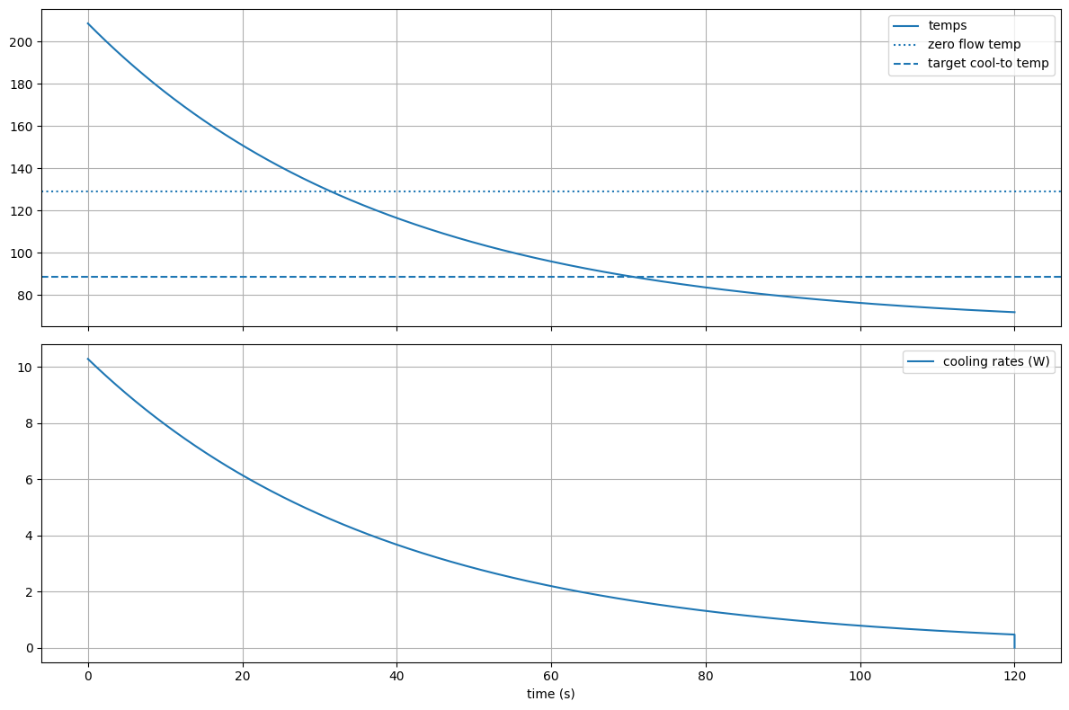
We can work out a cooling time constant \(\tau\) using Equation 7.8, and an equilibrium temperature \(T_{eq}\) using Equation 7.9. Finally, we use these to calculate the layer cooling time, \(t_{min} (s)\) with Equation 7.10.

\[ \begin{aligned} \tau = (C) / (h_{air} + h_{layer}) \end{aligned} \tag{7.8}\]

\[ \begin{aligned} T_{eq} = \frac{(h_{air} \cdot T_{ambient} + h_{layer} \cdot T_{targ})}{(h_{air} + h_{layer})} \end{aligned} \tag{7.9}\]

\[ \begin{aligned} t_{min} = -\tau \cdot log((T_{targ} - T_{eq})/(T_{noz} - T_{eq})) \end{aligned} \tag{7.10}\]

This model is approximate, for example our equilibrium temperature calculation assumes that the previous layer’s temperature is a boundary condition, when of course it actually continues cooling into the layer below it as time progresses. This means that we probably over estimate layer cooling times. Our model could be extended across each layer, but we would need to develop a much more complex (and probably geometric) solver for this - the approximation works well enough especially considering that we are already estimating \(h_{air}\) and the filament’s conductivity.

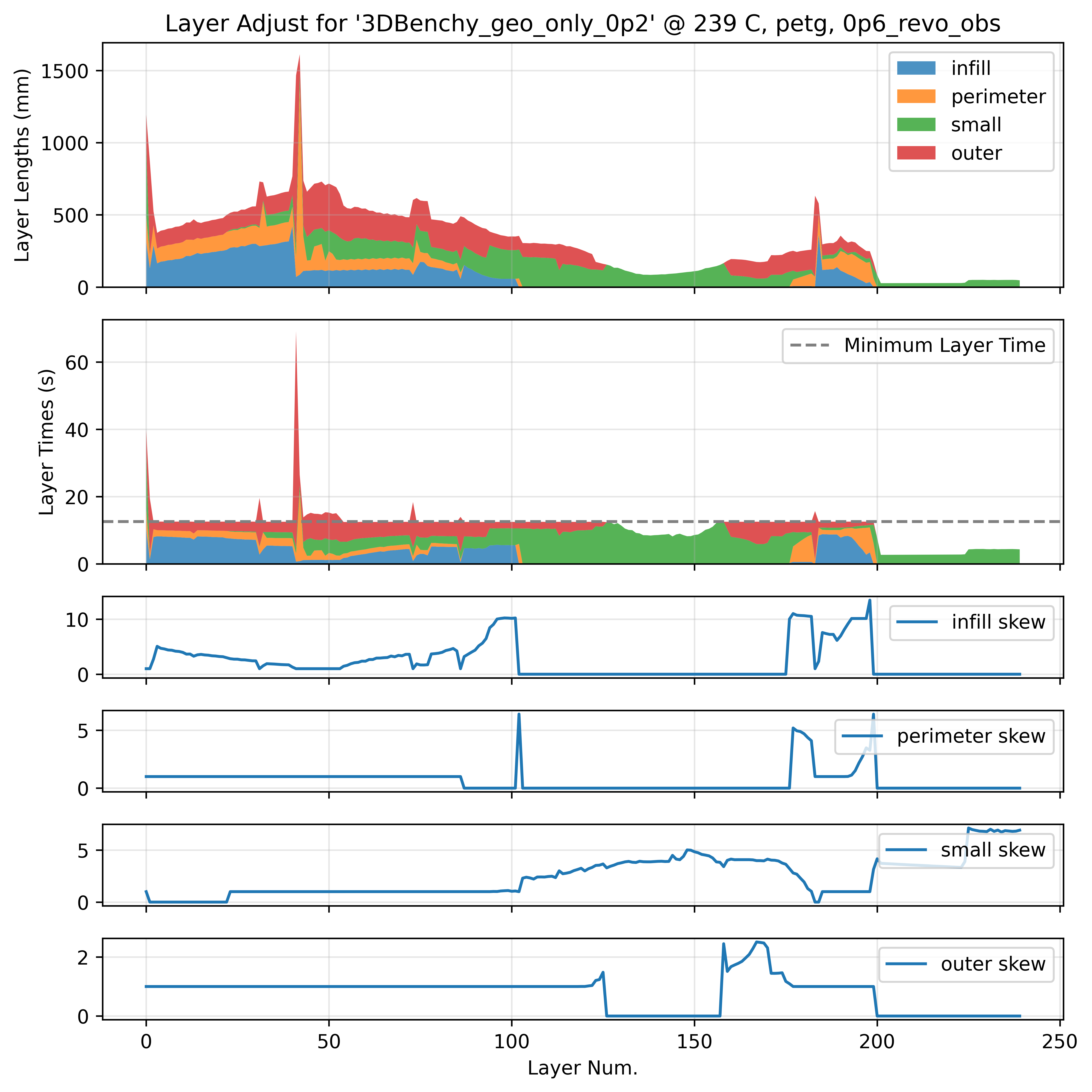
Above: a time-series simulation of the layer cooling system for PETG, including target temperature and the material’s zero flow temperature. Below: power flow out of the layer, in Watts.

7.4.3.3 Adjusting Segment \(V_{max}\) for Minimum Layer Times

To enforce minimum layer times, we assign maximum velocities to segments within each layer. This is simple enough: in small layers with times shorter than the minimum, we squish the velocity to extend the time. However, we prefer to skew velocities in segments that are less critical to our overall dimensions and appearances, i.e. the infill is modified first, if this does not suffice we move to the perimeters, and if this is still not enough we modify the external perimeters. This insight comes from Prusa Research’s note on the topic (Prusa Research 2024): polymer tracks extruded at higher speeds / pressures have slightly different visual properties (more matte) than those printed at lower speeds (which tend to be glossier). They also have different rates of die swell (see Section 7.3.6). Finally, we have a global limit to the skew, such that no segments have a translational velocity of less than \(10mm/s\).

Figure 7.21: This figure shows layer-by-layer (horizontal axis) segment lengths (top row) and times (second from top), colored by segment types: infills, perimeters, small perimeters, and outer perimeters. To meet a minimum layer time (horizontal dashed line, second from top), rates for these segments are skewed: skew proportions are plotted for each category in the bottom four rows.

This visualizes the layer skews in the figure above in a 3D plot. Most of the skewed segments are within the infill.

7.4.3.4 Optimal Nozzle Temperature for Minimum Print Times

So by now we can pick a viable temperature range from some minimum up to the nozzle’s maximum, and then at any temperature we can select flowrates for each segment type, and calculate and then enforce a minimum layer time. Having done all of that work, we can pretty easily pick a nozzle temperature that will give us the minimum total print time.

This optimization turns out to be exceptionally simple and intuitive. In smaller parts, total print time tends to be dominated by the minimum layer time and so colder nozzle temperatures (less cooling) are preferred. As parts increase in size, print time is dominated more by the flowrate / time to actually deposit the layer - so we want to increase the temperature to increase these flowrates.

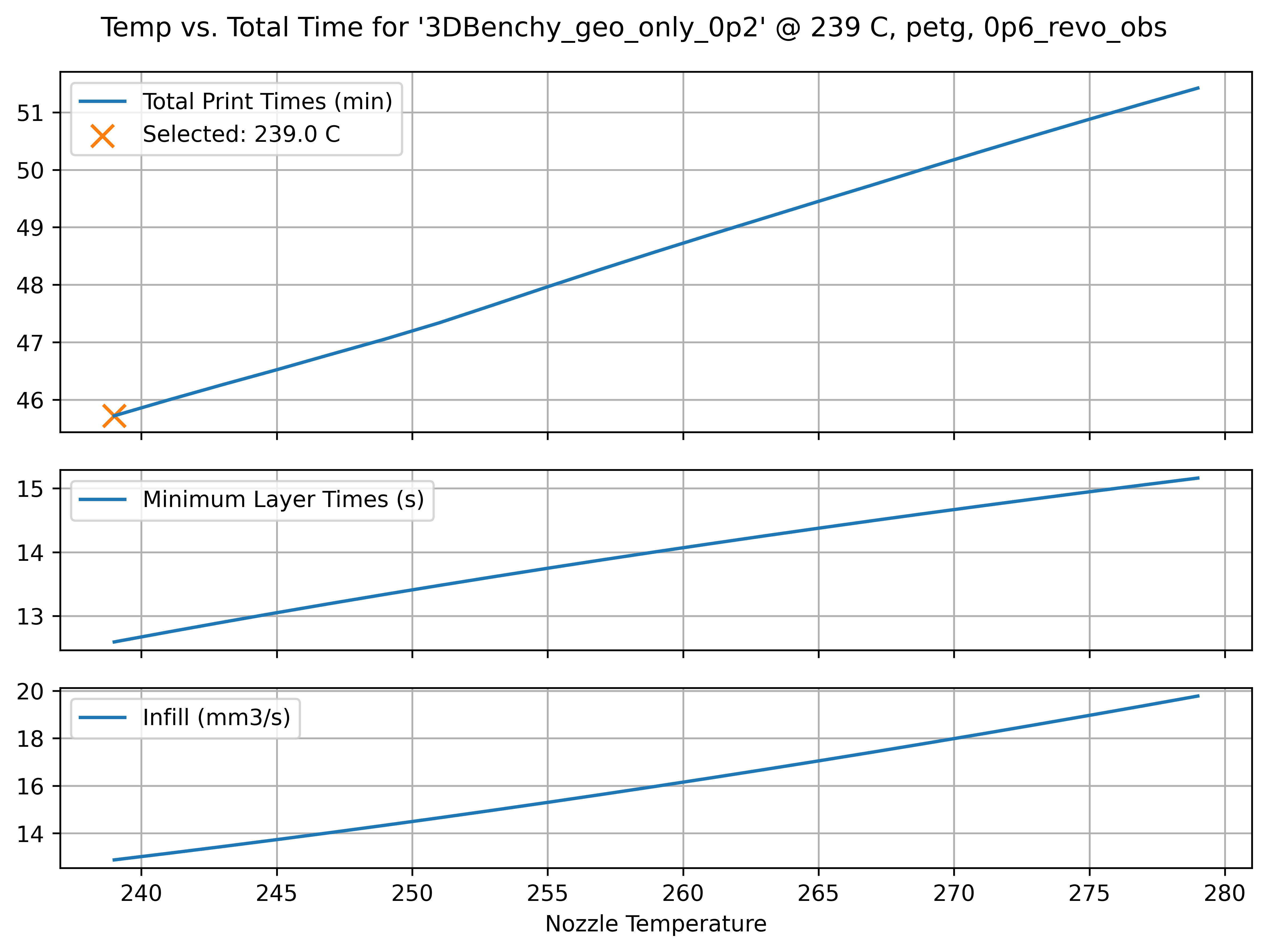
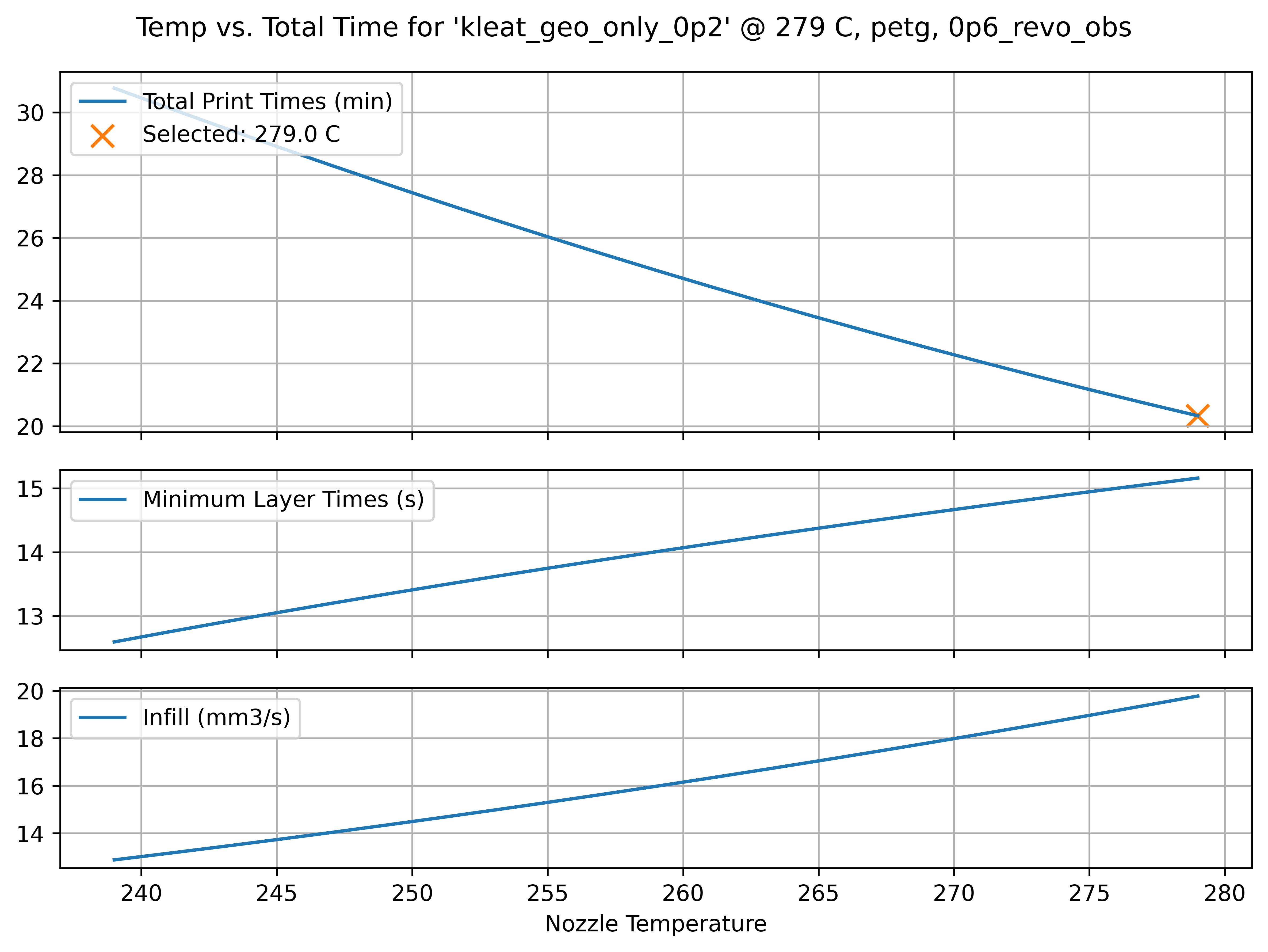
Figure 7.22: For the 3DBenchy (top) and the Rheo-Printer’s toolchanger plate (bottom), we see the total print time across temperatures, as well as the minimum layer times and infill flow rates (left plots). The benchy (~60x30mm) has a minimum print time at the minimum nozzle temperature, while the plate (~60x80mm) has a minimum print time around the maximum nozzle temperature.

There is a crossover print size that depends on our cooling models, i.e. in the Rheo Printer with PETG (and a 0.6mm Nozzle) I found that prints about Benchy sized (60x30mm) clearly favour cold flows, whereas even slightly larger prints (90x70mm) clearly favour maximally hot flows (Figure 7.22). Parts in between exhibit a clear optimum temperature somewhere between our minimum and maximum temperatures. In these cases, flowrates and layer times increase together and balance such that the average layer time naturally meets the minimum layer time (Figure 7.23). If we increase our estimate of the printer’s cooling capability, the crossover size gets smaller (and vice versa). For polymers where temperature increases don’t lead to exceptional gains in flow, colder temperatures overall are preferred, etc.

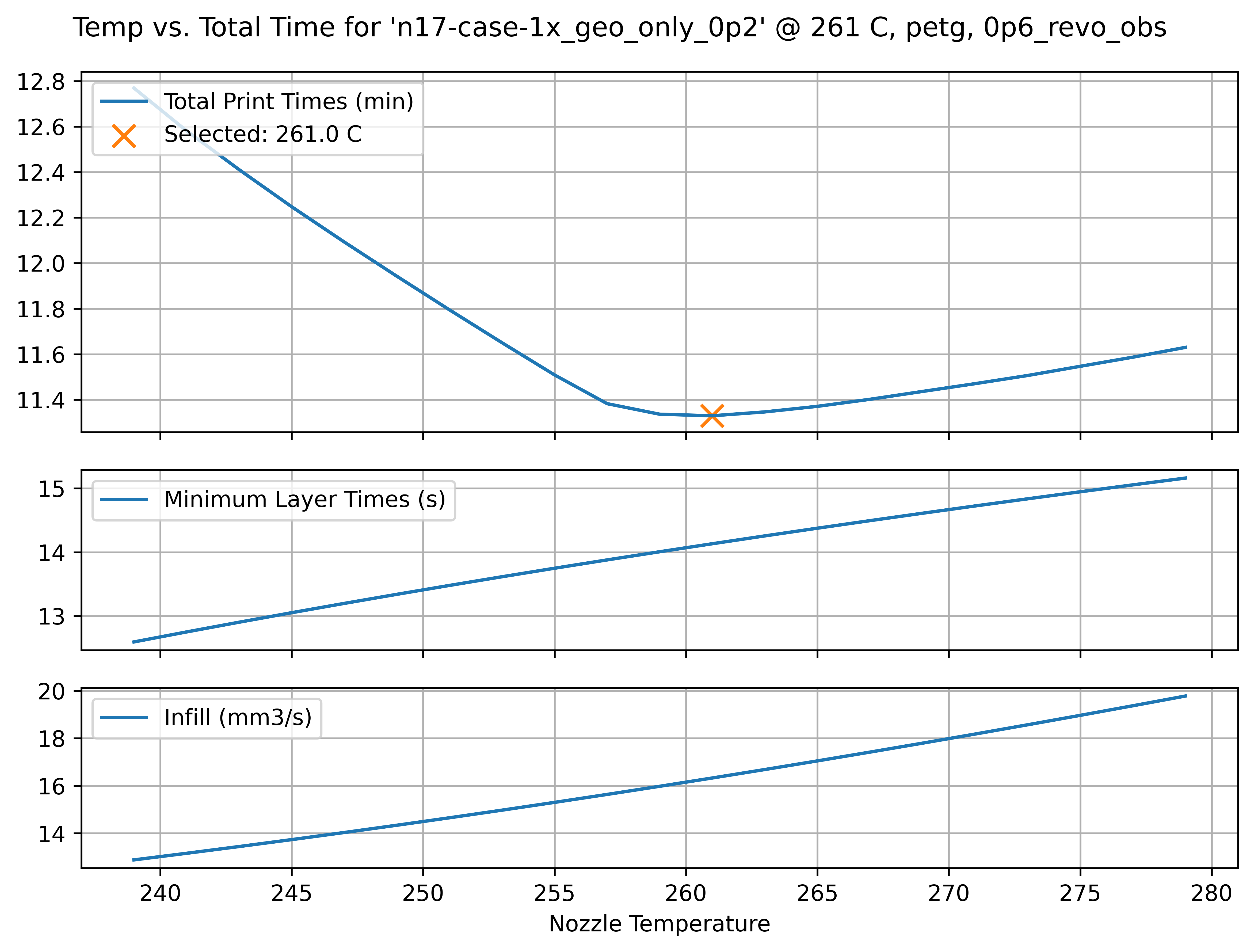
Figure 7.23: This part (a circuit enclosure, right) has a layer size that is in the crossover range for optimal print times (~40x40mm). The optimal temperature for the best total time (left) emerges as a clear minimum.

I had always thought that printers were over-optimized for producing small, detailed parts. The 3DBenchy is the de-facto parameter tuning object partially because it encapsulates lots of different features but also because it prints relatively quickly which decreases the loop time for tuning iterations. However, we typically print larger beds with i.e. multiple small parts or larger single parts. This basically means that print which have been hand tuned tend to favour colder temperatures overall, even though there are huge speed gains to be had by increasing the nozzle temperature, i.e. we can select a very hot flow for the larger part in Figure 7.22 (second row) that decreases the total print time from 30 minutes to 20 minutes. In the case of this work, because we develop print parameters over the entire range of viable temperatures, we can more flexibly adjust that single parameter and let our models and “meta heuristics” dial out the rest of the knobs.

7.4.3.5 Future Development of “Pareto Frontier Printing”

The key tuning knob in the optimum nozzle temperature step is picking our target layer temperature \(T_{targ}\) - if we favor “hot and fast” prints that may be somewhat slumped (but stronger), we can dial this up: the minimum-time optimization will be penalized less for warmer flows (as minimum layer times will be shorter). If we want precision above all, we can turn this down and we will see the opposite result. This makes up one axis in a theoretical pareto frontier, which trades strength (at the cost of precision) for speed.

TODO: maybe actually do a prototype of this: ternary plot w/ images of 3DBenchy in each corner. Need to “model” layer adhesion… but could get hand wavey.

While I do not develop this, could formulate trade-offs for precision, speed and layer strength by defining optimal results for each. Optimal speed is obvious: we measure total time. Overall precision is a strong function of our cooling target (and overall flow speeds, slower flows being more predictable). Layer adhesion / part strength is a function of the layer interfaces’ thermal history, which I have shown can be modelled ~ basically just using layer times (we just need to integrate interface temperature over time). What is missing from the current work is a characterization of how much layer strength is gained from a given increase in interface temperature / time, and how much precision is gained from slowing down and over-cooling parts. However, I think that good heuristics could be developed in these cases, and the literature contains a slew of studies on each topic.

We could also develop this more completely to scan a print from bottom to top layers, analysing an ideal temperature for each layer such that print speed is maximized while the layer is sufficiently cool before the next begins. For example a print with large layers near the bottom and small near the top should begin with large nozzle temperatures and slowly cool as it approaches the small, detailed sections. This would require models not only for part cooling, but for the available thermal ramp rates of the nozzle. New printers are also being developed that use induction heating of the nozzle which greatly reduces thermal mass and enables much faster thermal response. These could be exploited to very quickly change nozzle temperature layer-to-layer or even feature-to-feature in a print. Lookahead solvers that account for short-term dynamics (acceleration, pressure) and longer-term dynamics (thermals) could presumably be developed to suit.

From here, I think the future of FFF printing is bright - I know that there are many others working in this domain, and (luckily for the public good) many of the bottlenecking patents have expired⁵. Despite the onslaught of new strategies being developed for additive (laser bed fusion, binder jetting, etc etc), FFF remains extremely useful, relatively easy, cheap, and (as we see here and elsewhere) capable of producing excellent parts whose performance is similar to injection moulded components (and using the same low-cost materials).

7.4.4 A Note on Slicing with Models

The preprocessor that I developed for this task is awkwardly placed between a traditional slicer (which I use to generate path geometry only), and our controller (see Figure 7.4). I hope it is clear that the broader proposal is not to add a step, but instead to integrate these models into state of the art slicers. We could even take this one step further and integrate the slicer with the printer’s motion models, etc. Taken to its conclusion, this approach also enables optimizations on path geometry, i.e. choosing to increase print density where users select strength over speed, etc etc.

7.5 Real-Time Planning with Motion and Flow Models

(from proposal… intro ?) As I discuss in Section 7.1, Section 8.1 and Section 1.4.1, much of the work that machine users need to do to operate digital fabrication equipment is an implicit optimization. In this thesis, I try to make that optimization explicit, and base its operation on models that are generated in-situ on the machines in question.

prior chapter’s motion planning algorithm, plus a simultaneous simulation that does extruder pressures/dts -> extruder motor currents, inflows, didt…
cost function evaluates against target flowrate/mm, so as soln’ to velocity is developed, target flows / mm shift…

Figure 7.24: This is a plot generated from the online optimizer I have written that solves for the Rheo-Printer’s motion system and polymer flow simultaneously, using models as shown in Listing 6.1 and Listing 7.2. At left, we see the simulated trajectory, with arrows color-coded to resulting velocity at each time step and with target extrusion (light grey) with resulting extrusion (dark grey). This simulation is differentiable with respect to a cost function that describes *optimal* control outputs as those which maximize printer velocity while minimizing errors. At right, various output plots from the same simulation; errors (top), solver gradients, solver torques (middle) and velocities (bottom). The solve is done over a quarter-second receding horizon window, with one time-step’s control outputs (4 milliseconds long) issued each cycle.

The approach shares much in common with Model Predictive Control, which is a common approach to control for dynamic robots (Di Carlo et al. 2018) - here we show that when we use models that are developed in situ, the same pattern can be applied to machine processes.

I will evaluate the success of this contribution by comparing the printer’s dimensional performance, as well as its speed, to a converntional workflow and machine. I will also compare the amount of user input required for successful prints using this method vs. using traditional workflows.

We come to the meat of the problem! For years I shared a dream with my fellow machine builders at the CBA and elsewhere that we could use motion models and flow models together to optimize motion trajectories in some digital fab machine. I turned to optimization based solutions with the suspicion that “almost anything” could be articulated in a cost function, and solved optimally as a result. Working out an exact formulation that would be successful was the challenge.

This turned out to work, in a miracle of computation that means I can finally graduate. In the last chapter, I discussed how the motion solver works in phase space to pick velocities across many linear segments, and then calculates the required (vs available) actuator currents in each of these segments. We can do the same trick for the extruder system.

We have alredy discussed our flow models, where nozzle pressure and temperature relate to flowrate. In the formulation used in this work, the solver’s decision variable is simply the target pressure, which is very directly related to the actual output from the system.

The solver picks speeds vs at each line segment, which can be combined with the trajectory’s target flowrate per mm to generate a target flowrate for the interval. Then we have the challenge of relating the pressure time-series to the states that generate that pressure: extruder velocities and the currents required by the extruder actuator to generate those velocities (and pressures).

I characterize the extruder motor using the same workflow as outlined in the previous chapter, and get a model of the voltage to current dynamics (which limits motor jerk), and the current to torque (and acceleration, velocity etc). The extruder system needs to move the mass of filament (another inertia), which is subject to some damping, and it has the additional dynamic that a steady-state pressure requires a steady-state amount of torque to “push”.

To fit these dynamics, I use (TODO) a chirp (actually, TODO: I discussed this all previously, right?).

Using dts from the vs, we can run the same trick used in calculating the motion constraints for the system:

pi, pf at each step nets us two qi, qf flows (through that model…)
qi, qf w/ dt nets us the total cubic mm that have flowed out from the nozzle in this interval,
flow_out + d_pres make for a total amount of inflow that needs to be generated across this step,
this generates the inflow time-series,
current required by the extruder at this step is related to inflow + the current:pressure scalar we discussed earlier.

(From the proposal) At the time of writing, models are defined in my motion controllers by writing authoring integration functions. Provided that these are purely functional, they can be combined easily into the gradient-descent based optimizer that I have developed with JAX (G. Research 2024), a differential programming library. This integrator here describes how the Rheo-Printer’s position changes over time, depending on commanded motor torques, it is ‘half’ of the system that we want to optimize in order to operate the machine.

Listing 7.2

def integrate_flow(torque, inflow, pres, del_t):
    k_outflow = 2.85        # outflow = pres*k_outflow 
    k_tq = 1                # torque scalar, 
    k_pushback = 10         # relates pressure to torque 
    k_fric = 0.2            # damping 

    torque = np.clip(torque, -1, 1)

    # calculate force at top (inflow) and integrate for new inflow 
    force_in = torque * k_tq - inflow * k_fric - np.clip(pres, 0, np.inf) * k_pushback
    inflow = inflow + force_in * del_t

    # outflow is related to previous pressure, simple proportional model for now
    outflow = pres * k_outflow

    # pressure rises w/ each tick of inflow, drops w/ outflow, 
    pres = pres + inflow * del_t - outflow * del_t

    # that's all for now?
    return outflow, inflow, pres

This has the effect of linking states in time, to generate a series of extruder motor currents required at each step. We additionally differentiate this current time series to get didt, and these are both plugged into the cost function (via softmax bounds), such that the solver finds a solution that does not violate the extruder actuator constraints. As discussed, we additionally add pressure constraints (where required) and maximum velocity constraints.

7.6 State-of-the-Art vs. Model Based 3D Printing

7.6.1 SOTA Prints vs. Our System: The Prusa Retrofit

Almost every component in the FFF controller (and machine) that I have developed here differs from the state of the art (SOTA): our controllers are modular, SOTA are monolithic. Ours are optimization and model-based, SOTA are heuristic and mostly feed-forward. During the course of the system development, I also used custom hardware in the Rheo-Printer.

As I have discussed, hardware limits are the real, physical constraint on FFF print speed and quality. So, to compare our controller to SOTA with different hardware wouldn’t make sense: it would be impossible to differentiate which results emerged from hardware design (which I am not studying here) and controller design and implementation. So, to make a hardware-to-hardware comparison, I retrofit a Prusa Core One printer with my controllers and implemented the FFF control stack described here on that machine.

This involved fitting motor and kinematic models of the printer using the workflow I described in Section 6.1 and Section 6.2, and then fitting flow models using techniques described in this section. The lynch-pin for me here is that the Prusa Extruder implements a loadcell into it’s design - primarily used by them for bed leveling - this is not available on all SOTA printers, but it is the most important flow modeling tool in our kit.

Besides the loadcell, I also added a microbolometer to the Prusa, since time-series thermal data is invaluable in print analysis. All other sensing is done indirectly using the motor controller’s current measurements.

Retrofit Prusa

Figure 7.25

Retrofit Prusa Extruder

Figure 7.26

Otherwise the modular controllers let us take over the Prusa hardware with relative ease; I use their power supply and connect it to two Knuckles Hubs, which then each connect to motor controllers, heaters, etc. Heaters are implemented using the HBridge Knuckle, and Low-Side Load Knuckle.

Retrofit Prusa PSU, Etc

Figure 7.27

Using this hardware, our comparisons bear more weight as we know that the ground truth physical constraints in our system are identical to those used by Prusa. It also gives us a set of print parameters to compare against, as they do an excellent job of shipping expertly tuned slicer parameter sets for their hardware.

So, armed with this comparison tool, I chose a range of filaments to develop models and test prints for. I chose a set that includes the incredibly common “defaults” like PLA and PETG (which are useful because they are well understood), as well as strange variants of the same (carbon-fiber reinforced, and high-temperature versions), because it is often difficult to ascertain exactly what these blends are and our system can operate well even with that uncertainty. I also included some high performance materials that are classically difficult to print like Nylon and PolyCarbonate-ABS blends (and both with glass fill), since these are excellent engineering materials and I was curious to see if our system could manage to learn how to print with them. Finally I included natural materials that are interesting for their renewable properties. For example NuTan is a material developed by a CBA Collaborator (vlasta?) (which is not commercially available yet as a filament), but is made from organic feedstocks - there are no presets available for NuTan, which may limit it’s real-world adoption, so I wanted to see if we could automatically develop these. Finally I included an Aluminum Fill material because I was interested to see a thermodynamic outlier; it’s conductivity and heat capacity should me much larger than other polymers.

For each of these materials I develop flow models - some with 0.4mm nozzles, and others (the filled materials) with a 0.6mm nozzle. I also printed a sample of parts to compare print times and (qualitatively) print quality.

7.6.1.1 0.4mm Nozzle Models

Key parameters for each, at min, max temps.

PLA, 0.4mm	\(\degree C\)	\(k\)	\(a_{sst}\)	\(b_{sst}\)	\(a_{iso}\)	\(b_{iso}\)
\(T_{min}\)
\(T_{max}\)

PETG, 0.4mm	\(\degree C\)	\(k\)	\(a_{sst}\)	\(b_{sst}\)	\(a_{iso}\)	\(b_{iso}\)
\(T_{min}\)
\(T_{max}\)

NuTan, 0.4mm	\(\degree C\)	\(k\)	\(a_{sst}\)	\(b_{sst}\)	\(a_{iso}\)	\(b_{iso}\)
\(T_{min}\)
\(T_{max}\)

Nylon, 0.4mm	\(\degree C\)	\(k\)	\(a_{sst}\)	\(b_{sst}\)	\(a_{iso}\)	\(b_{iso}\)
\(T_{min}\)
\(T_{max}\)

7.6.1.2 0.6mm Nozzle Models

PLA, 0.6mm	\(\degree C\)	\(k\)	\(a_{sst}\)	\(b_{sst}\)	\(a_{iso}\)	\(b_{iso}\)
\(T_{min}\)
\(T_{max}\)

HTPLA-CF, 0.6mm	\(\degree C\)	\(k\)	\(a_{sst}\)	\(b_{sst}\)	\(a_{iso}\)	\(b_{iso}\)
\(T_{min}\)
\(T_{max}\)

PETG, 0.6mm	\(\degree C\)	\(k\)	\(a_{sst}\)	\(b_{sst}\)	\(a_{iso}\)	\(b_{iso}\)
\(T_{min}\)
\(T_{max}\)

PETG-CF, 0.6mm	\(\degree C\)	\(k\)	\(a_{sst}\)	\(b_{sst}\)	\(a_{iso}\)	\(b_{iso}\)
\(T_{min}\)
\(T_{max}\)

Nylon-GF, 0.6mm	\(\degree C\)	\(k\)	\(a_{sst}\)	\(b_{sst}\)	\(a_{iso}\)	\(b_{iso}\)
\(T_{min}\)
\(T_{max}\)

PCABS-GF, 0.6mm	\(\degree C\)	\(k\)	\(a_{sst}\)	\(b_{sst}\)	\(a_{iso}\)	\(b_{iso}\)
\(T_{min}\)
\(T_{max}\)

Alu Fill, 0.6mm	\(\degree C\)	\(k\)	\(a_{sst}\)	\(b_{sst}\)	\(a_{iso}\)	\(b_{iso}\)
\(T_{min}\)
\(T_{max}\)

Wood Fill, 0.6mm	\(\degree C\)	\(k\)	\(a_{sst}\)	\(b_{sst}\)	\(a_{iso}\)	\(b_{iso}\)
\(T_{min}\)
\(T_{max}\)

7.6.1.3 Print Time and Quality Comparisons

Time, Image of each print to compare. Data will also be examined @ relevant modeling sections.

Benchy	Print Time	Image
SOTA, 0.4mm, PLA
Ours, 0.4mm, PLA
SOTA, 0.4mm, PETG
Ours, 0.4mm, PETG
SOTA, 0.4mm, NuTan	x	x
Ours, 0.4mm, NuTan
SOTA, 0.6mm, Wood Fill	x	x
Ours, 0.6mm, Wood Fill

Z Motor Mount	Print Time	Image
SOTA, 0.6mm, PETG-CF
Ours, 0.6mm, PETG-CF
SOTA, 0.6mm, Nylon-GF
Ours, 0.6mm, Nylon-GF
SOTA, 0.6mm, PCABS-GF	x	x
Ours, 0.6mm, PCABS-GF
SOTA, 0.6mm, HTPLA-GF	x	x
Ours, 0.6mm, HTPLA-GF

End Effector Plate	Print Time	Image
SOTA, 0.6mm, PETG-CF
Ours, 0.6mm, PETG-CF
SOTA, 0.6mm, Nylon-GF
Ours, 0.6mm, Nylon-GF
SOTA, 0.6mm, PCABS-GF
Ours, 0.6mm, PCABS-GF
SOTA, 0.6mm, Alu Fill
Ours, 0.6mm, Alu Fill

7.6.2 Reducing Parameter Spaces

Qualitative analysis: how many “decision variables” for traditional CAM vs. ours ?

Parameters… compression?

Figure 7.28

This section probably needs a good figure or two, to articulate ~ reduction of parameter spaces, and flexibility of movement w/ in those parameter spaces.

7.6.3 Learning from Printer Data Outputs

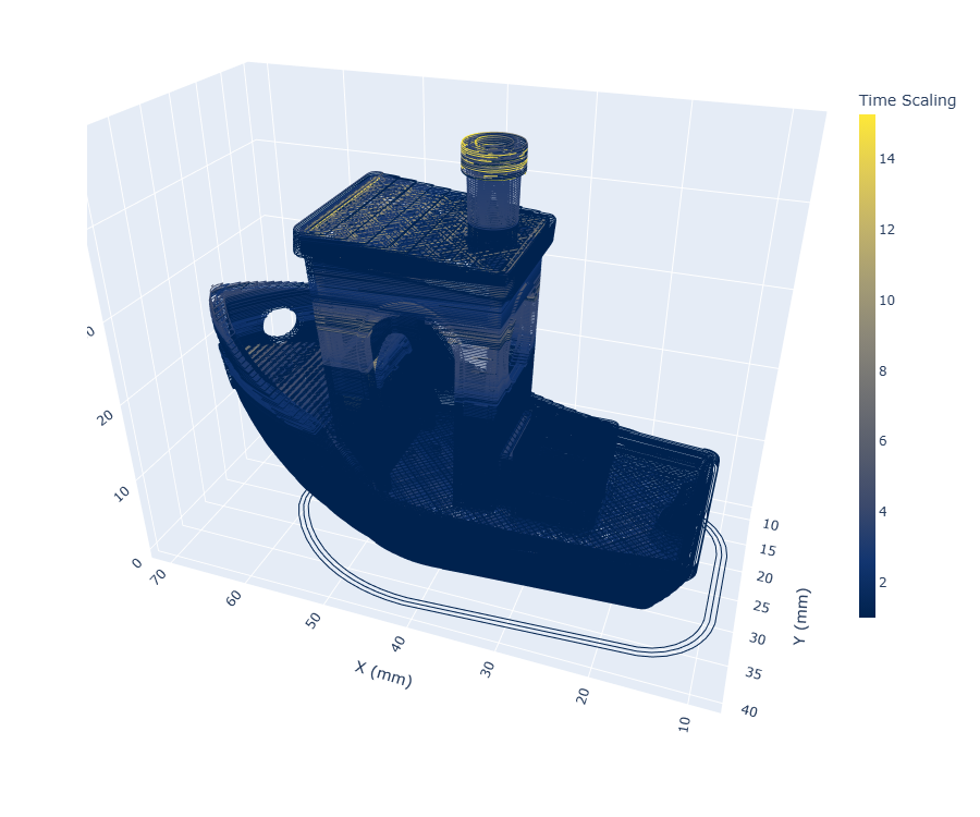
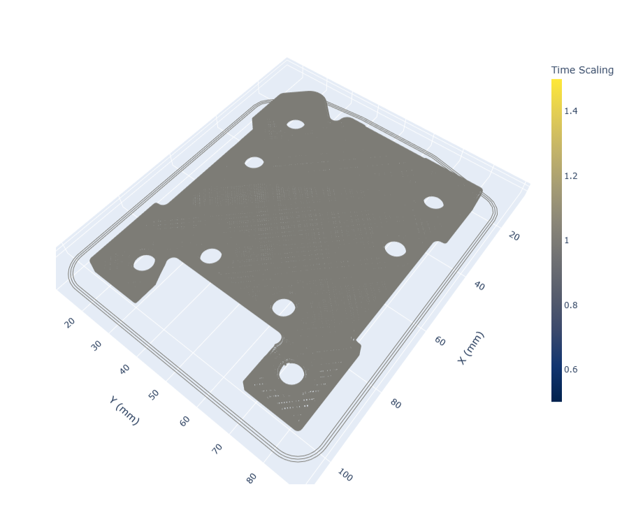
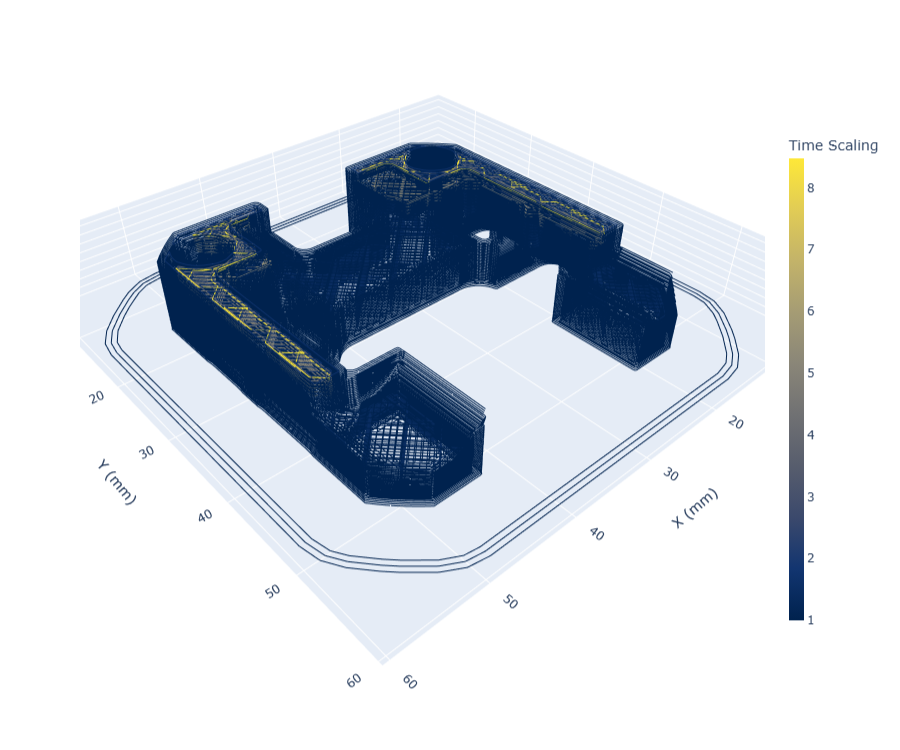
Whereas models on their own can tell us about how components of our system behave, the model based controller outputs can teach us about the system as a whole. During any print job, we collect numerous data streams from the machine and the solver that can all be used for analysis later - and with sufficiently accurate models, we can even do this with the system’s digital twin alone. Probably the most interesting way to process this data is to analyze (at every point in the part geometry) which aspect of the machine was limiting overall performance. This is shown below in Figure 7.29, where a few layers of a printed part are rendered with a colormap that corresponds to whichever system component was the most constraining on overall speed at that junction in the part. In Figure 7.30, the same data is rendered into bins showing how much time the printer spent during that job limited by each category.

The categories covered relate both to machine / motion models and flow models. Most dominant in this figure is cooling: tracks that have been slowed down to meet minimum layer time constraints. The second most dominant constraint are the flow models themselves, which are combined with some heuristics (recall Section 7.4). Then we have a series of machine related limits: inflow and inflow acceleration limits, as well as extruder current limits, are all related to the extruder motor’s performance and power budget. AB and Z motor current limits relate to our actuator’s performance, but also the machine’s motion system as a whole: reducing the occurance of these limits could involve increasing actuator size or decreasing friction or mass in the motion system.

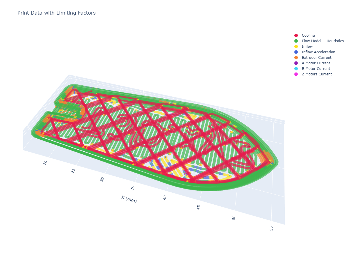
Figure 7.29: This figure renders a section of a printed part in 3D, with trajectory segments binned by whichever machine component (or model consideration) constrained the overall system speed at that segment.

Machine design is a game of trade-offs: if we improve overall flowrates by i.e. increasing the extruder motor size, we add mass that the motion system must heft around through tight corners. If we decrease the size of the part cooling fan to reduce that weight, we remove cooling performance and need to add more time in each layer to counter it. Actually determining which of these trade-offs is the best to make is difficult to ascertain on pen and paper (or with a good spreadsheet) alone, since it is difficult to understand how often our various constraints are the main limiting factor, and it is difficult to understand how they couple with one another. These limits are also geometry dependent: if we print small, intricate parts we are more likely to be limited by the machine’s motion system and part cooling - whereas large parts are more likely limited by overall flowrates.

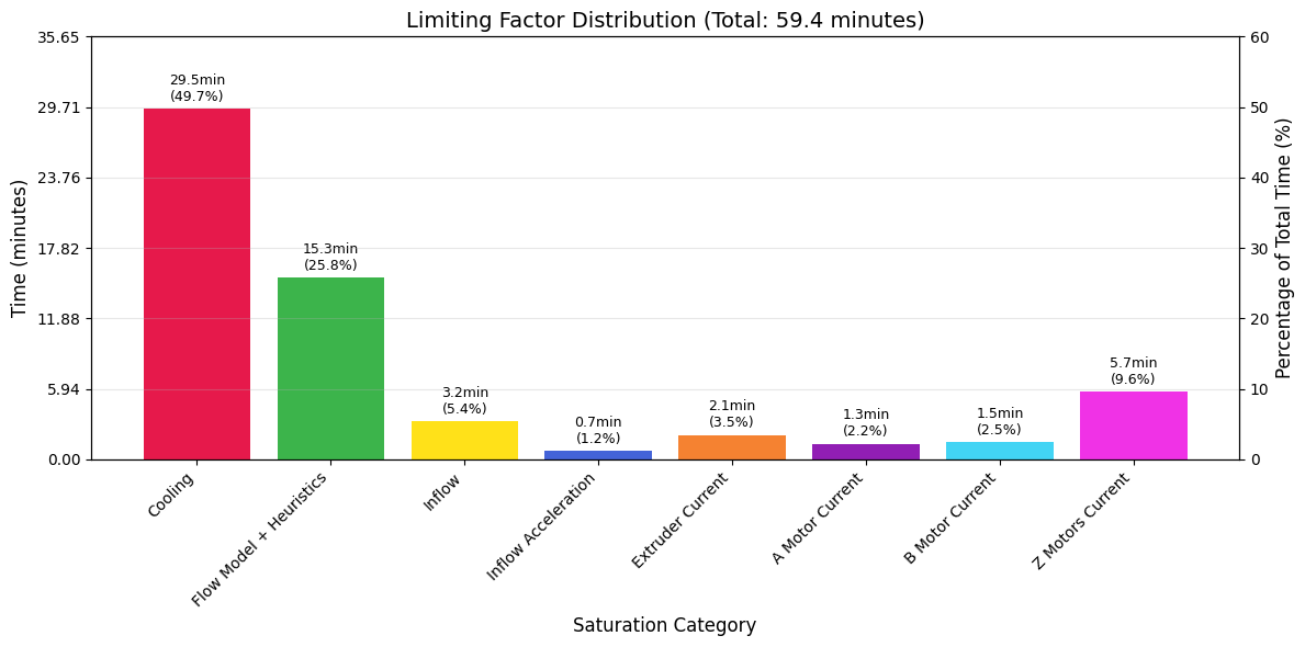
Figure 7.30: Here I show the total cumulative times that the printer spent during the job in Figure 7.29 limited by each machine component or model consideration.

Using outputs like this, which emerge from the solver’s optimization loop (and our models), we can learn directly how all of these systems relate, and help us to make better machine design decisions in the future. I want to connect this briefly to what I mentioned in the introduction. In the state of the art, all of this learning is done on a purely intuitive basis. We have very many inputs (CAM parameters) and only a few easily measured outputs (total part time and quality). To learn how the inputs (and machine components) combine to improve or degrade either of those ouputs takes years of tuning on our own internal mental models. With model based control, we can read internal states and outcomes and learn directly where and how much each of our decisions is impacting outputs, basically tightening the loop on heuristic selections and machine design choices. I want to stress that I do not see this as a replacement for our mental models of machines and processes, rather as a tool to help more of us develop those models in more detail, with less time, and in a manner that could be more easily shared with others.

To generate these outputs, we compare time series data of each component’s outputs state with the relevant limit, for example motor current utilization vs. the maximum current available at that time. Each segment has a maximum velocity set via flow models and related heuristics, when that velocity is saturated we know that nothing else is constraining speed - and when that velocity has been scaled to meet a minimum layer cooling time, we know that the part cooling model has limited speed at that point.

Besides this more complex binning of output data to determine limiting components, we can also render individual traces to learn about our system. I have included a few of the most interesting traces in the figures below.

Data output for nozzle pressure during a print.

Total filament “dwell time” during a print: how long the segment of filament currently being extruded has spent in the melt zone.

The vector sum of A and B motor currents.

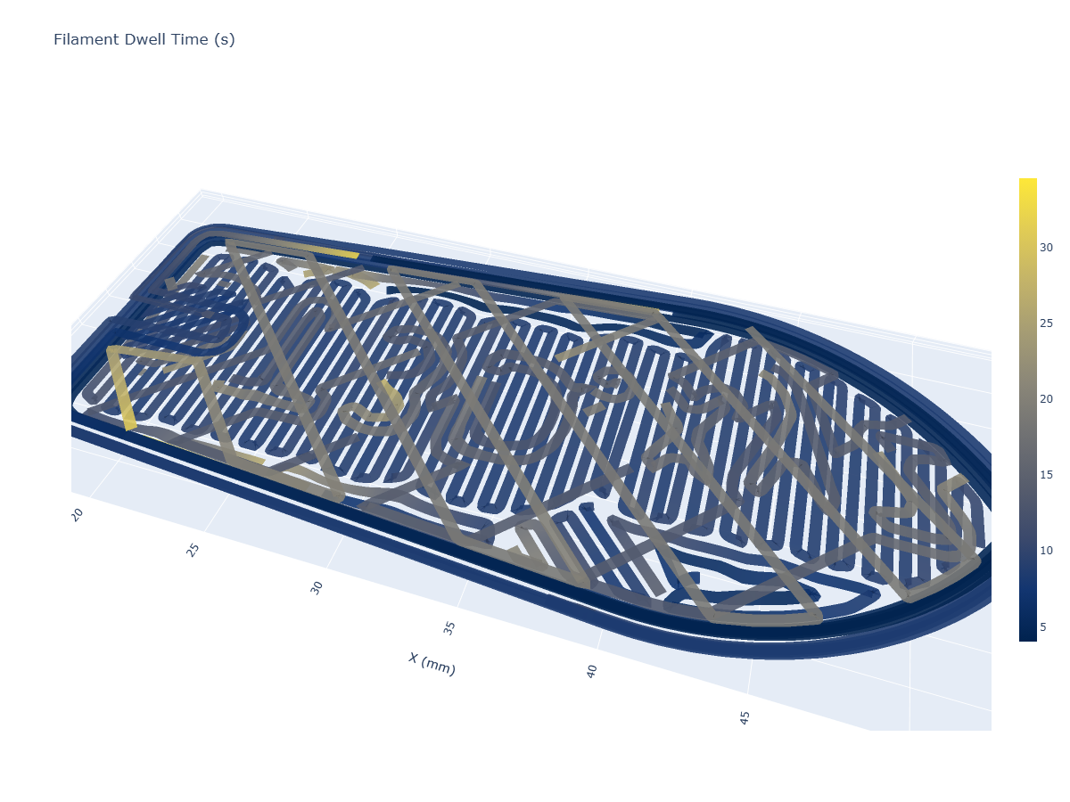
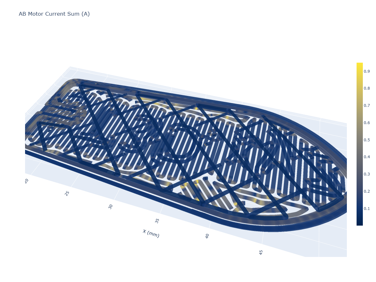
7.6.4 Learning from Flow Models

Writing and figure generation TODO here.
TODO: FIGURES / Table for a selection of materials.

In this section I want to explore what we can learn from flow models alone. We already discussed how flow linearity can help determine ~ melt points of materials and overall viscosities. Gaps between steady-state and isothermal models can tell us about our material (and nozzle’s) ability to transmit heat: bigger gaps are harder to heat, dadoi. Squish parameters are ~ probably proportional to material stiffness and softening rates, etc.

7.7 Continuous Improvement and Deployment

One of the things that makes this system unique is that the measurement equipment and the process equipment are the same. In most materials modeling paradigms, we use offline hardware to characterize samples, develop process parameters for feed-forward controllers, and then deploy them. In this case, we use much lower fidelity instrumentation but can use it continuously to generate “an embarrassment” of data (CITE: that paper Zimmer pointed out), which we can use to continually refine our system.

As we have seen, this has the primary advantage that the data is automatically aligned between the instruments we use to generate models and those where we deploy them (they’re the same instruments). This means that we can do an end-run around the many calibration steps that are normally required to align sensor data with SI units (so that models are transferrable across hardware).

For example the small thermal imaging device that we use is only precise within (5% ?), but it is consistent with itself. These thermal camera measurements are also highly dependent on the emissivity of the object being measured: in this case, we can eliminate this uncertainty by simply making … new models for each variable filament, basically removing the offset by using relative values (?). The loadcell is similar: it generates signed 24-bit integer readings which we calibrate to real values in Newtons, but this step is not explicitly necessary: we want only to know how the reading ultimately relates to flow from the nozzle.

Calibrations aside, the real power of using local instruments for control is that we can use data generated on the machine during normal operation to continuously refine models….

Motion Current Error with initial Inertia and Damping Estimates

Motion Current Err. w/ J, k_d fit from in-process data.

Figure 7.31

Figure 7.32: **Click here for a video.** Earlier in Figure NUM we looked at data collection for steady-state FDM model building, in this figure we see a screenshot from a data collection routine on the Rheo-Printer where dynamics data are being collected form the loadcell and filament sensor, time-synchronized to the motion controller’s states. At the time of writing, we can collect dynamical flow data from the first layer only due to our relatively naive computer vision setup - a major part of the next step in this research arc is to outfit the printer such that we can collect high frequency data at each layer.

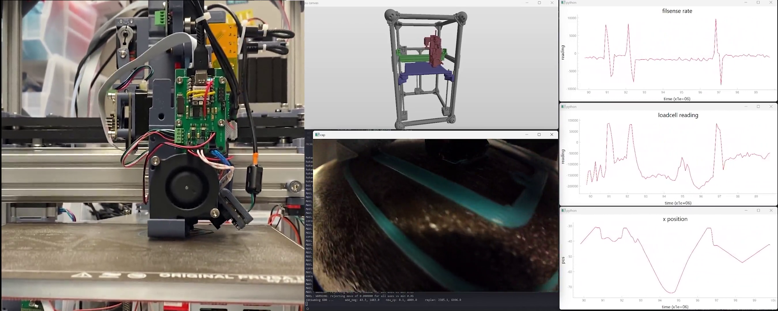
after any given print, we can update models with time series:
- what’s in the time series, and how do we weight it all ?
  - note that pressure from these tests is probably noisy due to nozzle-whacking-stuff,
  - thermal ? images are probably very instructive…
- not sure yet how much of this can be done…
- these go back to… stored model .pkl’s ? with which parameters ?

7.8 Future Work

… lots we missed, do we have the data to model it ?

… I’m sure there will be lots to say at this point: probably the biggest would be the ability to do a second planning step over the course of many layers, i.e. ramping temperatures in larger layers, dialling back in smaller layers… (there is some new work on this from others)
- want to show that the data we generate (thermal history) can be used to tune those heuristic parameters intelligently, and to understand print outputs more completely, i.e. predict inter-layer adhesion… and ~ maybe offer a tuning handle for strength vs. speed more directly…
… pellet extruders…

7.8.1 Forwards Simulation Based Solving

it’s easier to write dynamics down as time-series / ODEs - unfortunately for this solver we have to manually transcribe from those representations into “backwards” looking models. bummer, and it seems like other MPC solvers don’t have the same constraint: so what’s up with that?

References

Afonso, João Araújo, Jorge Lino Alves, Gabriela Caldas, Barbara Perry Gouveia, Leonardo Santana, and Jorge Belinha. 2021. “Influence of 3D Printing Process Parameters on the Mechanical Properties and Mass of PLA Parts and Predictive Models.” Rapid Prototyping Journal 27 (3): 487–95.

Coogan, Timothy J, and David O Kazmer. 2019. “In-Line Rheological Monitoring of Fused Deposition Modeling.” Journal of Rheology 63 (1): 141–55.

———. 2020. “Prediction of Interlayer Strength in Material Extrusion Additive Manufacturing.” Additive Manufacturing 35: 101368.

CreativeTools. n.d. “3D Benchy.” Free STL Model.

Davis, Chelsea S., Kaitlyn E. Hillgartner, Seung Hoon Han, and Jonathan E. Seppala. 2017. “Mechanical Strength of Welding Zones Produced by Polymer Extrusion Additive Manufacturing.” Additive Manufacturing 16 (August): 162–66. https://doi.org/10.1016/j.addma.2017.06.006.

Deshwal, Sandeep, Ashwani Kumar, and Deepak Chhabra. 2020. “Exercising Hybrid Statistical Tools GA-RSM, GA-ANN and GA-ANFIS to Optimize FDM Process Parameters for Tensile Strength Improvement.” CIRP Journal of Manufacturing Science and Technology 31: 189–99.

Di Carlo, Jared, Patrick M Wensing, Benjamin Katz, Gerardo Bledt, and Sangbae Kim. 2018. “Dynamic Locomotion in the Mit Cheetah 3 Through Convex Model-Predictive Control.” In 2018 IEEE/RSJ International Conference on Intelligent Robots and Systems (IROS), 1–9. IEEE.

Ferretti, Patrich, Christian Leon-Cardenas, Gian Maria Santi, Merve Sali, Elisa Ciotti, Leonardo Frizziero, Giampiero Donnici, and Alfredo Liverani. 2021. “Relationship Between FDM 3D Printing Parameters Study: Parameter Optimization for Lower Defects.” Polymers 13 (13): 2190.

Go, Jamison, Scott N Schiffres, Adam G Stevens, and A John Hart. 2017. “Rate Limits of Additive Manufacturing by Fused Filament Fabrication and Guidelines for High-Throughput System Design.” Additive Manufacturing 16: 1–11.

Kazmer, David O., Austin R. Colon, Amy M. Peterson, and Sun Kyoung Kim. 2021. “Concurrent Characterization of Compressibility and Viscosity in Extrusion-Based Additive Manufacturing of Acrylonitrile Butadiene Styrene with Fault Diagnoses.” Additive Manufacturing 46 (October): 102106. https://doi.org/10.1016/j.addma.2021.102106.

Luzanin, Ognjan, Dejan Movrin, Vassilis Stathopoulos, Pavlos Pandis, Tanja Radusin, and Vera Guduric. 2019. “Impact of Processing Parameters on Tensile Strength, in-Process Crystallinity and Mesostructure in FDM-Fabricated PLA Specimens.” Rapid Prototyping Journal 25 (8): 1398–1410.

Mackay, Michael E. 2018. “The Importance of Rheological Behavior in the Additive Manufacturing Technique Material Extrusion.” Journal of Rheology 62 (6): 1549–61.

Mackay, Michael E, Zachary R Swain, Colby R Banbury, David D Phan, and David A Edwards. 2017. “The Performance of the Hot End in a Plasticating 3D Printer.” Journal of Rheology 61 (2): 229–36.

Prusa Research. 2024. “New in PrusaSlicer: Consistent Surface Finish and Nerfing VFAs on the CORE One and Other Printers!” Prusa Research Blog. https://blog.prusa3d.com/new-in-prusaslicer-consistent-surface-finish-and-nerfing-vfas_120400/.

Qattawi, Ala, Buraaq Alrawi, Arturo Guzman, et al. 2017. “Experimental Optimization of Fused Deposition Modelling Processing Parameters: A Design-for-Manufacturing Approach.” Procedia Manufacturing 10: 791–803.

Read, Jake Robert, Jonathan E Seppala, Filippos Tourlomousis, James A Warren, Nicole Bakker, and Neil Gershenfeld. 2024. “Online Measurement for Parameter Discovery in Fused Filament Fabrication.” Integrating Materials and Manufacturing Innovation 13 (2): 541–54.

Research, Google. 2024. “JAX: Autograd and XLA for High-Performance Machine Learning Research.” https://github.com/google/jax.

Research, Prusa. 2024. “PrusaSlicer: Open-Source 3D Printer Slicer Software.” https://github.com/prusa3d/PrusaSlicer.

———. n.d. “Linear Advance in FFF Printing.” https://help.prusa3d.com/article/linear-advance_2252.

Sanladerer, Thomas. 2021. “InFiDEL Filament Sensor.” Printables Design Files. https://www.youtube.com/watch?v=RYgdLPe_T0c.

Turner, Brian N, Robert Strong, and Scott A Gold. 2014. “A Review of Melt Extrusion Additive Manufacturing Processes: I. Process Design and Modeling.” Rapid Prototyping Journal 20 (3): 192–204.

Wu, Pinyi. 2024. “Modeling and Feedforward Deposition Control in Fused Filament Fabrication.”

The “benchy” boat has become the de-facto test print in the FFF development community, probably because it contains a swath of difficult to print features (like overhangs and bridges), is small enough to print quickly, and because it is cute.↩︎
One of the all time great modelling anecdotes is Norbert Wiener’s “The best material model for a cat is another, or preferably the same, cat,” - as in, messy systems are best modelled by themselves. This is kind of the point of the machine that measures its own models, but the counterpoint is just as valuable, and it takes the form of Borges’ small story On Exactitude in Science which is itself quite small, I can even just copy paste it in here, check it out: “…In that Empire, the Art of Cartography attained such Perfection that the map of a single Province occupied the entirety of a City, and the map of the Empire, the entirety of a Province. In time, those Unconscionable Maps no longer satisfied, and the Cartographers Guilds struck a Map of the Empire whose size was that of the Empire, and which coincided point for point with it. The following Generations, who were not so fond of the Study of Cartography as their Forebears had been, saw that that vast Map was Useless, and not without some Pitilessness was it, that they delivered it up to the Inclemencies of Sun and Winters. In the Deserts of the West, still today, there are Tattered Ruins of that Map, inhabited by Animals and Beggars; in all the Land there is no other Relic of the Disciplines of Geography.” … The point being that no, a complete model is not useful, because it does not do the thing that we want models to do, which is to reduce a complex thing into a simpler representation that we can understand. OK.↩︎
The subreddit in question is reddit.com/r/FirstLayerPorn.↩︎
Side note: developing an intuition for the Watt is a valuable engineering practice… recall that a typical incandescent bulb is rated to 100W and about 95% of those Watts are coming out of the bulb as heat energy… probably don’t touch it directly, but sticking your hand close to the bulb will give you a sense for the amount of energy that “100W” is.↩︎
For example Stratasys held a patent on enclosed build chambers and so for about 15 years most FFF companies couldn’t put their machine in a box (which greatly improves part warping, and makes the printer less susceptible to i.e. a drafty room). Some readers may be wondering why I keep calling it FFF - well, the other acronym is trademarked by the same company. This is all fair game in today’s patent law ecosystem, but a clear case where our old laws (developed in an era where technological advancement was more costly and took place in longer cycles) have become outdated. Not to mention a changing global order, especially in manufacturing, where some of the main participants are developing equipment within completely different legal frameworks - given the difference in the two worlds’ approaches to IP law it is no surprise to me that they are able to innovate at such an outstanding pace. Notes should be taken…↩︎