7 Discussion
In the introduction I posed a set of guiding questions about machines (1.6). The particular answers are spread across the chapters above; it is worth summarizing here how each was answered and pointing back to where each was demonstrated.
To the question of systems architecture for feedback-based machine control, Section 2.3 looks at how heterogeneous networking enables the networking of high- and low-level machine control components, and Section 2.4 shows how that can be combined with software representations of controllers which can be rapidly reconfigured. Using networks and networked software components rather than file formats (like GCode) enables us to build machine workflows across planning and control steps. Describing workflows that combine variable control configuration steps alongside machine tasking is then managed by combining dataflow representations with scripting capability, which allows us to easily switch between machine configurations as testing devices (to build preliminary models) and as output devices (to make parts). I showed that the systems can be re-configured (rather than re-built) to develop both 3D printing and CNC machining controllers (5.4, 6.4.1), as well as a collection of pen plotters (2.7.5.1) and various other ad hoc machine projects.
On the question of what a complete feedback-based digital fabrication workflow might look like, Section 5.3 develops one that is mostly complete. It is missing the trajectory generation step, but builds processes for both high- and low-level planning using models alongside explicit optimization. The result is a substantially reduced parameter space that must be tuned by hand (5.10.3).
On the question of what models we need to capture machine physics, and whether we can build them using the machines themselves: Section 4.4 describes a motor controller that can fit its own models (4.5.1), and Section 4.5.2 shows how kinematic models (4.3.2) can be fit from machine data. In Chapter 5 I show how models for polymer melt flow (5.5) and print cooling (5.7) can be developed that combine machine and material physics together using computational metrology. In all of these modelling examples I use the machines where the models will be used to build the models. This is enabled by the systems architecture mentioned above, and greatly simplifies the deployment of model-based control because models are automatically aligned to hardware. Other model-based approaches require an “offline loop” where models developed using e.g. SI-unit specifications must be carefully calibrated for use across many pieces of hardware, each of which has its own small variabilities (4.8.4).
Reframing machine control from the state-of-the-art’s implicit constrained optimization (one solved by operators using tacit knowledge) into an explicit, numerically solved one, Section 4.6 shows that velocity planners — where state-of-the-art solutions are already explicit formulations — can be improved by replacing heuristic parameters with high-fidelity motor and kinematic models. This enables our planners to utilize more of our motion systems’ underlying dynamic range, which enables faster overall processing rates (4.7.1) and shows promise to noticeably improve the productivity of CNC machining (4.8.1). In 3D printing, the optimization-based workflow lets us move more fluidly around in process parameter space which, when coupled with high-level optimizations, leads to decreased printing time compared to the state-of-the-art — especially for larger parts (Section 5.10.4).
In the introduction I also expressed some concern that model- and optimization-based approaches could turn productive processes into black boxes, hiding the intuition that operators and designers already bring to their machines. In Section 5.10.3 I show how workflows that use explicit optimization steps need not become black boxes, by developing techniques that let us mix heuristics with models (5.8.1). In 6.3.1 I showed how virtual machines can be used as a tool for CNC operators to virtually compare toolpaths’ velocity deviations (~ deviations from their target chip loads), and to estimate cutting forces from machine data (6.3.2). To demonstrate the use of these tools I combine them with my own tacit knowledge to iteratively develop a machining toolpath in Section 6.4.3. The outputs from our planners are themselves informative: we are after all producing lots of process data every time we use these machines. In Section 5.11.3 I show how process models can teach us about materials, and Section 5.11.1 shows how planner- and machine-sourced datasets can teach us about our hardware’s limits and how they interact with process geometry and parameters.
Finally, on the question of how models might be used in machine design, Section 5.11.1 (above) doubles as a designer’s feedback tool, and Section 6.4.2 demonstrates how models can be applied by designers in their selection of motors and motion parameters for heuristically tuned velocity planners.
7.1 Crossing the Gap: Partitioning Machines
The introduction to this thesis discusses how today’s machine control systems partition (split) dynamical operation of hardware (in GCode interpreters) from planning (in CAM and slicers). Relevant background sections covered how this is largely still true even in state-of-the-art research efforts and in distributed systems architectures for robotics. This results in simple problems like computational misconfigurations where systems-scale programs don’t have ground-truth knowledge about what devices they are co-ordinating. It also leads to more complex lossiness issues where high-level planning steps don’t understand what will really happen when their plans are sent to hardware (or what that hardware is capable of / constrained by).
In Section 1.4.1 I explored the economic-scale reasons that even out-of-date partitions remain “sticky” in industry, and Section 1.4.2 describes the underlying technical limits that drive partitioning; those are mostly explained by network timing and computational constraints. Those both lead to a situation where most systems are partitioned across what I called the “realtime gap” between high- and low-level computing. But these split representations — and GCode in particular — prevent us from addressing machine control as a constrained optimization problem. Doing that requires that we connect low-level physical models to operation across scales, Section 1.5 explains why making that connection is a key goal in this thesis.
To cross the gap, Chapter 2 rebuilds machine control as set of distributed system modules; components in both high- and low-level systems are both first class citizens here. The new architectural tools here combine patterns from simple embedded networks for spacecraft with patterns from larger, messier and more reconfigurable systems on the web. Section 2.4 overlays programs in those networks to combine dataflow with scripting for configuration and control, and Section 2.5 builds core, reusable motion control software modules in that framework. This mixes fast, stateless operation with smarter high level configuration in an attempt to build high performance and deterministic systems that span the gap and are also reconfigurable.
These tools don’t eliminate the partitioning problem; parts of machine controllers need to run in embedded devices and parts should run in workstation-scale computing. But they build machine controllers in such a way that the partitions and networks are exposed within the systems description itself rather than hidden in abstract data layers and static interfaces. In Section 2.8.5 I argue that this takes an important step towards the assembly of systems design tools that can express systems design itself (not just machine operation) as a kind of constrained optimization. That would be an improvement over the state-of-the-art, where re-configurability of embedded systems is perhaps not limited by software architectures and interfaces themselves, but by our inability solve the scheduling problem when it is spread across many layers and modules.
The flexibility inherent in the architectures that I built enables me to assemble complex systems, for example bootstrapping model-based control by building simple, single-device models and tests and then sequentially assembling them into higher-order systems (Section 2.7.2). Because we don’t change the underlying systems representation in these cycles, those assemblies remain editable and inspectable even once they are “complete;” the result of the transformation is not to replace GCode with some new language or representation, it is to expose underlying representations in a unified and more navigable way: we go from GCodes to just Codes (Section 2.7.3).
That means that we can rapidly reassign hardware for different tasks my modifying software-defined controllers, for example using machines both as process modelling tools and as process operation equipment (Section 2.7.4). It also means that we can reconfigure software and hardware modules for new applications, i.e. use the same set of MAXL blocks, circuits, networks, and motion planners and models in both FFF 3D printers, CNC milling machines, and other ad hoc machine projects (Sections 2.7.5 and 2.7.10).
Although the architectures that I built are designed to represent “almost any” partitioning scheme, there are still some key limits (Section 2.8.1) in that regard. Section 2.9 explores how an expanded set of tools in this framework would enable more heterogeneity in this regard, but in this work I mostly locate high-level tasks (velocity planning, system configuration, and tasking) on workstation-scale computing in Python scripts.
Locating the majority of a machine controller’s description and state in the operating system has some major benefits; we can deploy much more computing there (Section 2.7.8), and can more easily expose important internal control states (Section 2.7.6). Both of these properties are critical when we move on to apply model-based control directly to machines. When we do apply model-based methods here, we can use literally the same model definitions (in .py files) across fitting, tuning, and control steps because each of those take place in workstation-scale computing.
Doing so requires that the realtime gap is crossed carefully because operating systems are inherently non-deterministic; Section 2.5.2 on the “MAXL Gap” explains how I do this. I trade some bottom-line bandwidth performance for determinism; a fixed-gap, fixed-interval trajectory computing and transmission system makes for consistent network and compute loads, and both can be configured against performance measurements made using the system itself. I explored that idea in the section that measures the architecture’s network and compute performance (2.7.9) and connects those measurements to MAXL’s bottom line performance (which still surpasses bandwidths reported by other state-of-the-art model-based machine control researchers, see Sections 2.7.9.1 and 2.7.9.4).
7.2 Wait, it’s all Models?
Always has been…
The first and second halves of the thesis (systems, and then models) at first feel somewhat unrelated, each living in distinct fields (rheologists rarely think about embedded computing), but really they both try to address the same problem: that machines are poorly represented in the state-of-the-art, as I discussed in Section 1.3.2.
Since we are talking about representation in both cases, of course the theme of modelling connects the two halves. It is not a new idea that machines could be represented computationally: there is much talk about using digital twins for this purpose. The trouble is that twins can easily diverge from their real-world counterparts; misconfigurations between real and virtual worlds can easily emerge when twins are defined by hand / from the top down. This makes subtle differences hard to identify and correct.
I have tried to articulate in a number of places that manufacturing is messy and why machines are heterogeneous in nature. Trying to homogenize systems with rigid top-down definitions is bound to cause more errors than it solves; in Section 1.4 I provided a few real-world and very costly examples. Instead, I think that we should try to design systems that help us (humans) reflect on and manage that complexity based on feedback.
In both halves of this thesis, I drive model building with bottom-up discovery; this means that alignments are automatic and misconfigurations can be detected against the real ground truth, which is located in the world — not the hard drive.
7.2.1 As a Core Representation for Systems Integration
In the systems half, I built the Systems Object Model (SOM, 2.4.4.1: it’s like the browser’s DOM but for mechatronics). That provides a view of our machine’s programmatic layout, i.e. how each of the machine’s hardware and software components relate to one another over networks, and what dataflow links exist between each. In this step, I focussed on developing tools that source that representation from the systems themselves. Network maps and program configurations are discovered via graph traversals, and software definitions are managed via programming tools that reflect on source code itself rather than relying on the manually authored “interface description languages” (IDLs), which are common in other state-of-the-art distributed systems architectures.
These two steps ensure that the systems representations we author high-level configurations and tasks against are automatically aligned to reality — at least in so far as reality is defined by network, firmware, and software configurations. This greatly eases the programming burden on systems developers because they do not need to manually align high-level proxies to low-level firmwares. It also makes it easier to reconfigure systems because changes that may be required in lower level components can more readily be integrated by the application-specific controllers that will rely on them.
7.2.2 Computational Metrology
A good SOM may help us to make sense of how our machines works programmatically, i.e. how we talk to, configure, and task them, but it doesn’t make sense of what will actually happen when we do so. In Sections 1.1 and 1.3.1 I discussed how GCode-based systems struggle because of the heterogeneity that machine physics present; even if we can describe machines with more flexible APIs, this fact will not go away1 — even two motors with the same SKU can have meaningfully different characteristics (4.8.4).
The second half of the thesis addresses this heterogeneity by developing a set of physical models that represent dynamical behaviour computationally. A key idea in this aspect of the problem is to develop computational metrology, which James Warren, my advisors Neil Gershenfeld, and Jon Seppala, my colleague and fellow systems programming enjoyer Erik Strand and I explored in [1]. I have mentioned this in the thesis on a number of occasions, but should make it (and its value to us) explicit.
As in the systems half of the thesis where I try to source systems representations from systems themselves, here we are trying to source models of dynamical behaviour from machine physics themselves.
In computational modelling, we focus not on the development of e.g. SI-units based measurements of underlying material properties, but on fitting simulations to observed phenomenology. The difference can be subtle, but the models for polymer flow I develop in Section 5.5 are a good example; they predict system behaviour based on abstract internal models that correlate to rheology but don’t directly measure rheological properties like viscosity and shear rate. The insight is that models are for making predictions rather than measurements: in the example of 3D printing we don’t much care what our polymer’s viscosity is across melt flow temperatures, but we do care how flows will evolve over time.
In the state-of-the-art it is more common to measure material properties using offline / standalone equipment like rheometers and tensile testing machines, and then integrate those measurements into predictive models. Here we leverage the systems development work to combine sensing with operation and then fit models directly against behaviour. This basically amounts to skipping a few normalization steps: flow models for the RheoPrinter don’t make sense in the FrankenPrusa because they combine material and machine behaviour, but they don’t need to because both can build their own representations.
There are a few interesting results of the approach that are worth calling out. The first is that we can fit filament compressibility and flow against load cell force readings. I sometimes call that measurement “pressure;” it is analogous to pressure but is actually just a measurement of force applied to the filament by the extruder motor. In Section 5.2.3.3 I relayed how state-of-the-art systems rely on direct measurement of outgoing flowrate for this step; adding computational modelling allows us to remove these observations and instead fit against the internal state — we rely on models to connect flowrate from the nozzle tip to force and flowrate at the nozzle entrance; the models specify only that the system is internally consistent. In the earlier paper that I wrote using a similar measurement [2], these force readings were not even calibrated to Newtons, they were just normalized to the system’s max load.
Another printer-related example is in the cooling models. I apply computational modelling to data generated for the steady-state flow test to extract a measurement of a filament’s heat capacity (in Section 5.7.1). For the estimate for how cool the material should become before another layer can be printed on top, I use the flow models; each has a “zero flow temperature” that estimates the minimum temperature at which material can be extruded at all. Although that is not a direct measurement of the material’s glass transition temperature (where it becomes molten), it is a good proxy for how cold it should be to provide structure to the layer above. To combine them to estimate layer cooling time, I do add an extra step to normalize the heat capacity measurement in terms of real-world SI units \((J/mm^3)\). Here this is a required step because I connect that measurement to a cooling model that uses estimated values for heat transfer (into air and into the layer below) that are not “computationally modelled;” I rely on estimates from engineering literature that are relayed in similar units. In Section 5.12.3.3 I explore how the printer’s microbolometer (a small thermal camera) could be used to close the loop on these internal measurements using computational modelling to relate observed filament thermodynamics to both heating and cooling phenomena in the printer.
There are also the motor models. Torque curves are normally measured directly using dynamomemters: those are standalone devices that can apply bias torque to a motor while it is run through a range of speeds. Not everyone machine builder has one, but we all have motor drivers themselves. By deploying motor models here, we can replace the dynamometer with a simple disk of some known rotor inertia: models that estimate torque based on current (and against internal measurements for voltage and speed) can then back out the motor’s \(k_t,\) which correlates current to torque. These models are invaluable across just about every other machine modelling and control task in the thesis.
Having applied computational modelling to machines, the next subsections relay how I used them to improve dynamics planning and higher level process planning, and how they can provide feedback to machine operators and designers.
7.2.2.1 In Dynamics Planning
In representing machine physics using models, we can more easily describe dynamics planners that optimize over those models to control hardware, rather than encoding a separate set of parameters for those planners. Alongside the development of computational models for motion, this step also leveraged the systems architecture developments in the thesis (to apply big computing to the task) and required that I develop a unique planner formulation that expresses the problem in a manner that is computationally parallelizable (based on similar but slightly different formulations from the state-of-the-art in model predictive control).
A description of the planner itself is in Section 4.6, and in Section 4.7.1 I show that it out-performs a type of planner (based on trapezoids) that is common in the state-of-the-art. The performance gain emerges mostly because the model-based planner can plan against a rich description of the machine’s underlying constraints. Whereas other planners define per-axis maximum jerk, acceleration, and velocity parameters, this one uses models directly; those relay that e.g. motors have more torque at lower speeds and that machine friction helps us to decelerate.
I enumerated a long list of sophisticated motion control physics in Section 4.2.2 because the new planner formulation shows promise in solving over “almost any” motion dynamics that we can articulate via computational modelling. I show this directly by extending it to solve flow models for FFF 3D printing in Section 5.9. Section 5.11.5 shows that the planner can produce solutions even against the time-varying nozzle thermodynamics present in the printer’s rheological system and Section 4.9.2 explores how similar time-varying physics in motors themselves could be included in future versions. I compare the planner’s printing speed with the state-of-the-art in Section 5.10.4. It is faster, but it is difficult to say if in this case the speed-up was due to model-based control or was instead based on other higher-lever choices made by the workflow that I developed there. Section 5.11.7.1 calls out the lack of clear evaluation across components in the printer chapter as an overall limit to the work.
Using model-based velocity planning in a formulation where internal states of the planner are exposed also has the effect that running the machine is tantamount to simulating the machine; because the models used by the planner are sourced from hardware, we operate the machine with the same digital twin that describes it. The systems architecture allows us to flexibly deploy software on variable hardware; to run an offline simulation this just means modifying a systems configuration to include no hardware.
7.2.2.2 In High Level Planning and Tuning
Models can also be used piecewise in higher level planning and configuration / tuning steps. Whereas I developed machine models primarily with the goal of deploying them in optimization based dynamics planners, I was surprised to find that they show huge value in these steps. Because new dynamics planners are currently less deterministic than their state-of-the-art counterparts, these may be more immediately applicable results in terms of broader adoption of the work in this thesis.
The basic insight is that models let us select operating parameters with respect to real underlying constraints, whereas state-of-the-art workflows are based on “guess and check” workflows. Modern CAM tools use direct parameters to describe how machines should operate but don’t relay to users how those parameters (which are directly encoded in GCodes) relate to physics. In Section 5.8.1 I develop a method for selecting machine speeds and flowrates against flow models using heuristically defined proportions of underlying physical limits. Rather than specifying how to operate and guessing whether this will exceed machine capability, we declare that operation should operate at e.g. \(90\%\) of its maximum flowrate for infill zones in a print and \(50\%\) of its maximum during more detailed parts. This is applied to motion control as well by regulating deployment of motor currents.
Those selections can then be combined with other optimizations against physics, the dynamics planner is the obvious example (it constrains against dynamical limits whereas selected parameters describe steady-state parameter selections alone), but I also provided the example in Section 5.8.4 of selecting nozzle temperature with a combination of cooling models and heuristics-and-model-based flowrate parameters. This combines declarative operation with computation that can select otherwise unconstrained parameters, Section 5.11.4 shows why leaving e.g. the nozzle temperature itself as a free parameter can lead to substantial speed-ups in printing.
I argue in Section 5.11.2 that this is a better way to combine tacit knowledge about machine dynamics with computational control of those dynamics. Instead of throwing parametric darts at the machine constraint wall, we describe the subset of viable parameter spaces that our intuition tells us the machine should use in particular zones and leave the rest up to intelligent algorithms. This shows up also Section 6.2.2 for the CNC milling machine, where I select motion parameters for a classical trapezoid-based velocity planner using models.
Methods like this also greatly simplify the task of machine operation, Section 5.10.3 shows clearly how the end-to-end feedback-based printer control workflow that I develop reduces the space of parameters that must be selected by hand. Those parameters — as I’ve just mentioned — are also mediated by models, so one intuitively developed set can be “broadcast” against new physical configurations.
To subsequently develop that intuition, the new tools that I built also enable us to visualize rich outputs from our hardware once we have run jobs (or before we do). Section 5.11.1 shows this most clearly: underlying physical limits in hardware are overlaid on printed (or simulated) trajectories to connect machine physics with process outcomes. We can use these data to understand why certain approaches work and others don’t, and also to understand why errors occurred; see Section 5.10.5.1. I show how these may be used in CNC machining as well in Section 6.3.
In this work I don’t engage in any path planning optimizations; each of the systems I work on operates based on trajectory geometry that has been defined in existing state-of-the-art tools. In the printing chapter I ingest GCodes from slicers, strip them of all but the geometric operation, and develop the process parameters and dynamics control on top of that and in the machining chapter I run my systems only for velocity planning and operation of the machine (and data collection). Section 7.7.1 briefly describes how the models and methods here could be used directly by — or extended to become — path planning algorithms that are also model-based.
7.2.2.3 In Machine Design
In the very beginning of the thesis I was making a workforce development argument; the new control systems we build should help more people become machine builders as well as users. The systems development chapter is most directly related to this because it is explicitly oriented around the way that machine controllers are assembled, reconfigured etc. But the tools that I’ve just described also have a natural relation to machine design: if we can express machine operation directly in relation to underlying physical constraints, it becomes more obvious how machine design decisions relate to operation. A goal there is to provide machine users with the thread they need to pull on so that they might become machine builders.
That is, we operate machines against their physical constraints and design them in an attempt to remove or minimize as many of those constraints. But it is often difficult even to sophisticated machine designers how all the decisions that they make will ultimately relate to bottom line performance. This is especially true when machines will interact with a heterogeneous set of materials and be used to make a highly variable set of part geometries; machines that work well to make small detailed parts (where precision above all is important) may perform poorly when tasked with fabricating larger, simpler geometries (where total power deployable is more important).
So, the outputs that I showed in Section 5.11.1 (on “Learning from Machines”) have obvious utility for machine designers too. I also showed in Section 5.11.3 how flow models can be used to understand materials and nozzles in more detail. In the CNC machining chapter I drew up a much more explicit example of this, using in Section 6.4.2 a set of model-based tools to select motors for an existing CNC machine kit. With models of my own motors and the particular hardware that I had assembled, I was able to push the machine’s performance well beyond what the kit manufacturer recommended.
7.2.3 Over Machine Lifespans
Model based control is probably an excellent basis for the maintenance and monitoring of machines over their lifecycles as well; in Section 4.7.3 I quickly showed that data collected from a machine can be used to improve models for control. Again, because the controllers work directly with those models, refitting models is equivalent to updating controllers to reflect changes that have occurred during use. This is “continuous improvement and deployment” (CI/CD) for machines. Although the models that I use for polymer flows are formulated in a manner that makes this difficult to do for the 3D printing process, I discuss how they could be updated to remove this limit in Section 5.12.2. The work here already makes some progress in that regard because these machines can generate more data than they consume — in the printers this is about one gigabyte per hour (on plans that are encoded in a few megabytes); more data of course being an important basis for any future work on modelling.
This connects also to error detection, in Section 5.10.5.1 I showed that the areas where models are poorly matched to data clearly overlap with areas that printed poorly. That probably means that those areas represent state spaces in machine operation that were underrepresented in the initial data sets; operating machines in those regions naturally generates data to improve fits there. But once model fits are well established, areas where models disagree with data are more likely to predict genuine out-of-band errors or disturbances; those could be used to identify and correct errors (potentially on-the-fly), or identify upstream changes, for example variable batches of input material or other unintended or unforeseen supply chain edits.
7.2.4 But Leave Room For Heuristics
I’ve already made reference to the application of additional heuristics on top of / alongside model-based control. Modelling is fundamentally about developing compressed representations: we use them to concisely describe complex systems. This means that good and bad models all miss some phenomenology. The models I develop here are no different, in particular the motion controller doesn’t understand machine vibration or stiffness and the printer workflow doesn’t really understand geometry, details about part cooling, and e.g. that outer perimeters should be more carefully printed than infill tracks.
If I had stopped to develop models for each of these aspects of the problem I would never have finished this work; where models miss it is important to be able to still use heuristics. Developing the methods that I deployed to mix heuristics with models was some of the most interesting work perhaps specifically because they are somewhat non-rigorous and simultaneously the most useful. In some sense this is the same point to the one I just made in Section 7.2.2.2; because there are so many competing concerns in machine design and control, simpler approaches or distillations of that complexity can be more valuable than making attempts to exhaustively map2 them.
In other cases, using heuristics for control can be preferable because they are simple and interpretable in terms of the outputs that they generate even though their input parameters are set directly. A trapezoid based velocity planner will not tell us why our machine can’t move faster than \(100mm/s\), we know that it will because that is the limit that we manually configured it to. Alongside the computing constraints that I have discussed, this is perhaps another reason why state-of-the-art industrial controllers (see Section 4.2.6) are still configured against direct parameters rather than models and solvers.
But again models are not incompatible with these systems, we have the methods that I have described which mix heuristics with models, and also the work I’ve described that uses models to select those direct parameters (6.2.2). We can also overlay models on plans that were generated using these more classical planners, as in the section in the machining chapter where I estimate cutting forces (Section 6.3.2).
7.2.5 With Regard to Economic Partitions
In the introduction I mentioned the economic partitioning problem (Section 1.4.1) and its relation to GCode’s pervasiveness: systems integration must happen across firms who each develop parts of an integrated system. Where internal representations of those systems are difficult to see or edit, integrations are harder and existing partitions and formats become stickier [3].
In modular or networked control systems we have a similar challenge; control components are developed by many firms and they each have the challenge of exposing their contributions to systems integrators. For technically complex components that are tightly integrated into other systems this is ultimately about explaining how the components work. The standard practice here is to write a datasheet [4], i.e. a document that explains some of the component’s inner working model, how systems integrators should expect it to function in certain states, and how they can interact with it (over which protocols, accessing which memory fields etc.). These documents can be extensive, for example the manual for Delta Tau motion controllers (a state-of-the-art modular motion system) is over 800 pages long [5] which represents a clear burden for systems integrators: presumably they will have to read it.
Ultimately this step is about reaching from the component’s actual implementation (engineering work done within the firm) through a compressed representation of how it works (the datasheet) and back into another integrated system. Datasheets are sometimes lossy for the same reason that other manually authored configurations are: reality as defined in the implementation can diverge from what was last written down. In industry, companies who develop a particular device are sometimes purchased by other firms who then subsequently move or modify these documents: they become inherited artefacts and the original engineers who authored them may be long gone at the time of their use.
I hope that this work’s relevance here is clear: the systems in this thesis base schema collection on discovery, which is subsequently based on automated tools that scrape schemas directly from source code. That is, I try to reach directly from the implementation layer to the description layer to ensure consistency across both. The world of software design does not include datasheets (especially where source code is open source) because well written software APIs convey enough information. It helps that computing is much more homogeneous than hardware: that makes operation of those APIs more predictable. But again, I am proposing that these dynamical models can help in that regard.
The patterns that I deploy to collect data schemas from source code do exist in some software serialization libraries for distributed systems (see Section 2.6.1.1), but they have so-far not been deployed in hardware oriented systems. I would contend that they are more useful here exactly because of the economic and physical heterogeneity present in machine systems. We have not yet had access to the level of embedded computing required to bring them down this far the stack; they consume extra memory and compute cycles to run. The compiler tools that I used to build them (for “template programming”) are even somewhat new relative to the build systems used for most firmwares; I had to manually configure most of my firmware development tools to target these devices with more modern versions of C++. But that is changing; microcontrollers are faster and cheaper than ever and languages like Rust are emerging as clear improvements over template-programming based strategies. In particular, open source hardware has a documentation problem; people who develop open hardware devices are burdened by the extra effort required to maintain it [6]. Developing discoverable schema in this way may help to ease that burden.
Overall, each of the topics that I have tried to cover for digital fabrication world are different aspects of one larger constrained optimization problem (see Section 1.5) which has many degrees of freedom. It is impossible to work on them in isolation, and it is difficult for individuals or individual firms who master one aspect to understand exactly how their contribution relates to the rest of the state-of-the-art. The machine control industry remains largely “partitioned;” a number of firms each offer complete and competing technological stacks that they protect with IP and secrecy [7]. For some time the computing industry was different, an emergence of standards for interoperation within computer systems led to what the authors of Design Rules Vol. 1 [8] call a “globally distributed, asynchronous systems design optimization effort;” competing firms all work together to produce components (CPUs, RAM, GPUs, displays, network interfaces, etc.) that are subsequently integrated into individually unique computers that remain globally addressable at the application layer via the power of code portability and computer science.
Key to that economic layout is the fact that component performance and specification can be easily relayed between firms. In this regard I would argue that models which are developed piecewise could fill a similar economic role. For example controls and CAM developers could virtually test their algorithms on a myriad of machine systems if those systems were well described as computational models or more complete “digital twins” (that include 3D models of hardware). In the same way, software developers can deploy their code on a litany of different computers via software virtualization; when the developer of an iOS app tests it, they often use a virtual iPhone. In the future work Section 8.1 I discuss the possibility of developing a standard for this purpose. Section 5.11.3 shows how models for flow can express dynamical performance of nozzles and materials, those are richer descriptions than the thin specifications currently provided by manufacturers of both and could help users and integrators make more informed decisions when choosing either. Good motor manufacturers already include torque curves for their products. Those can change depending on driver voltage and type, and a torque curve does not describe how the motor will integrate with (for example) another firm’s linear axis’ properties (inertia and friction). In Section 4.3 I show how piecewise models for each can be developed, and in Section 6.2.1 how they can be combined to intelligently select combinations of the two. I had to build those models, which required that I buy the machine kit and the motors to test. Providing computational models instead of datasheets could cut through some marketing layers and provide engineers with better tools for decision-making. I am not the first to imagine this type of economic layout, here I only want to draw the connection between the contributions that I did make in this regard and their broader impacts.
7.3 Wait, it’s all Connected?
A lot of the work in this thesis is oriented around the modularization of integrated systems. This is harder than simply building integrated systems that each do one specific task, except for the repeated labour that can be saved via those modularizations and e.g. the ability we then have to rapidly reconfigure the components into new systems. If the point of the thesis was simply to control 3D printers using feedback, all of Chapter 2 could seem somewhat irrelevant. Section 2.8.4 on OSAP and the OSI model is a start to this discussion: architects of the internet (which itself does not exactly follow the OSI model) make some points in an RFC that revolve around the reality that modularizations / abstractions can lead to inefficiencies and e.g. repeated computing steps because data hidden by one layer remains relevant in another.
This is an ongoing tension in systems design: abstractions are great except for where they fail, and in those cases they can be severely limiting. Whereas the work that I present here follows the end-to-end principle [9] in some regards, in reality decisions made at each layer were informed by my own understanding of constraints that emerge in others.
For example in Section 5.2.4.1 I shared how the FFF work in this thesis is primarily related to a line of research begun by TJ Coogan and David Kazmer, who developed an instrumented extruder similar to ours in [10] — it also adds a load cell between the extruder motor and the nozzle to estimate melt flow pressures. The key idea there is that we should be able to turn our processing hardware into process measurement equipment, i.e. use the extruder itself as a rheometer via computational metrology. Filippos Tourlomousis (a former collaborator) and Jon Seppala (one of my advisors) get the credit for bringing this idea to our research group at the CBA. Filippos built a prototype of the RheoPrinter’s hotend (Section 5.4.1) and I extended that with a design pattern developed by an FFF YouTuber to implement the filament sensor [11] (adding a feed rate encoder, and calibrating width measurements), and then began the long project of using that device as a tool to connect measurements to modelling and control.
This turned out to involve almost all the other work that I have described so far on improvements to systems architectures, motion controllers, and motor controllers. For example the closed-loop motor controller in Section 4.4 eventually supplanted the need for the RheoPrinter’s filament sensor and enabled me to develop a coupling between rheological models and the motors that drive them, the flexibility of MAXL’s basis spline representation (Section 2.5.3) was a key requirement for transmitting the complex motion instructions involved in nonlinear control of flow and MAXL’s piecewise assembly of motion controllers enabled me to run both model-building controllers on the RheoPrinter (which must be operable even when we do not yet have models) and the model-based controllers. OSAP and PIPES were key to all of this as connective tissue and to enable assembly of those piecewise controllers, and their flexibility allowed me to rapidly retrofit the FrankenPrusa (Section 5.4.2) in the later stages of this work in order for me to compare this new workflow to the state-of-the-art.
That is to say that I largely organized my systems design activities around a few core tasks. I tried to architect them such that they will be extensible in other use cases, but in reality that remains untested. I was able in Chapter 6 to rapidly redeploy them for a new machine and process (and they showed value there), and in Section 2.7 includes examples of a handful of other kinematic and ad hoc systems. Section 2.8.1 recounts the ways in which I anticipate that these architectural updates remain limited, but it is impossible to know for sure how developments or omissions I made there may limit other machine developer’s applications.
7.4 Basis Splines and Systems Assembly
In MAXL (Section 2.5) I use cubic basis splines (2.5.3) to encode motion. I discussed why these are useful with regard to the composability of various kinematics and other controls tasks in 2.8.2.
They do introduce some interpolation errors (I quantify those under the next heading) but they also relate neatly to constraints from our motion systems and our computational systems, which warrants some discussion.
7.4.1 Spline Errors and Motion Constraints
One issue with these splines is that they are not a direct interpolation.3 This represents some deviation between the control points that MAXL blocks transmit and the positions that motors actually interpolate through. In one sense the basis spline is a low pass filter on these points, which is an obvious problem for high precision motion control.
So, how much of a problem is it? Well, I would like to first point out that motion through a truly sharp corner at nonzero velocity requires an instantaneous change in velocity on at least one axis (an “infinite” spike in the acceleration of that axis),4 so we need to do some smoothing of linear piecewise paths or accept that our machines will flex and vibrate in unpredictable ways at these junctions.5 The better approach to the problem is to actually encode smooth paths according to a geometric tolerance, which is the basis of filter-based velocity planning approaches (see Section 4.2.5 and 4.2.8.2) but piecewise linear paths remain common in practice and in these cases encoding planned trajectories over line segments as basis splines actually helps because we eliminate these infinite spikes in acceleration from the curve which is followed by our hardware.
Still of course we would like to actually quantify the error. As it turns out, Delta Tau controllers6 also use basis splines to transmit motion to servo controllers. In their datasheet, they quantify the exact deviation error ([5] page 744):
\[ \text{Err} = \frac{V^2T^2}{6R} \tag{7.1}\]
Where \(V\) is velocity along the interpolated path, \(T\) is the timestep and \(R\) is the radius of curvature at the point of measurement. So if we take a relatively high speed and tight curvature \((V=500mm/s, R=10mm)\) and use the ~ four millisecond timestep that I used most often in the MAXL systems discussed in this document, we only see about \(70 \mu m\) deviation:
\[ \text{Err} = \frac{250000.0 \cdot 0.004096^2}{60.0} = 0.0699mm \tag{7.2}\]
In practice high speeds and tight corners don’t appear simultaneously; commercial 3D printers may advertise speeds of up to \(500mm/s\) but only ever achieve these velocities along straight paths - see for example Figure 1.7 in Section 1.3.3. Machines tend towards lower velocities in areas of high geometric complexities because cornering velocities are limited by actuator torque and machine stiffness7 so even if we blindly produce control points at a fixed time interval we end up packing more points into areas where geometries need more definition.
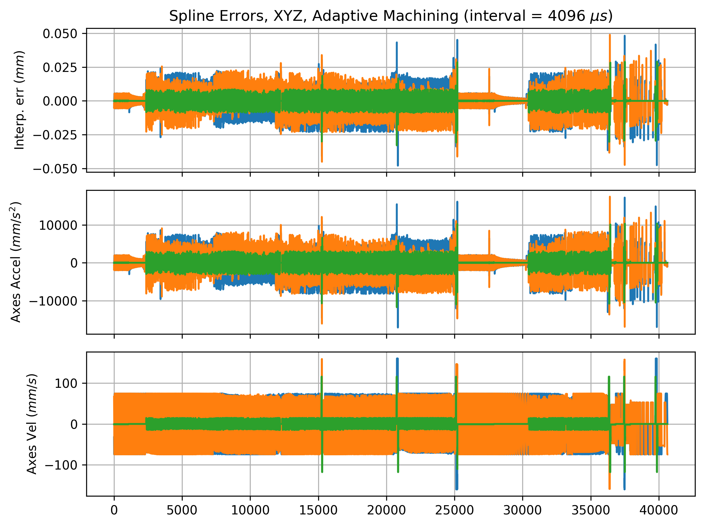
To show how this applies to real trajectories, I plotted interpolation errors along one of the planned CNC machining trajectories from Section 4.8.1 in Figure 7.1 below. These are measured numerically by taking the distance between each control point and the corresponding interpolated point.
7.4.2 Splines and Systems Integration Constraints
I think this discussion is especially interesting because it also relates to constraints from the systems integration perspective. For example some GCode interpreters work well with simple toolpaths but struggle with complex geometries that are encoded using very many small line segments. This happens for three reasons. The first is that GCode interpreters are often configured with a fixed number of segments in their planning queue whereas machine dynamics require that their velocity planners can see out to a minimum stopping distance. The second is that extra segments require extra compute to plan over. To ameliorate these issues most interpreters include a minimum segment length.8
The third pertains to network limits themselves in cases where we have to transmit GCodes from a host computer into the interpreter. While we don’t normally think of USB or SD cards as “network links,” both have real bandwidth limits.
For reliable control over networks we prefer to have deterministic network loads (Section 2.2.2.1) and using a fixed time interval accomplishes this. It also means that in the cases where we do need some buffering we can specify the size of that buffer against its real constraint which is time based,9 not spatial.
There is also a computational constraint at the terminal end of the problem where trajectories are actually actuated by stepper motors. To increase precision and smoothness of steppers modern systems use microstepping drives that interpolate full steps with smaller increments through the stepper motors’ electrical phases.10 At high speeds the stepping rate can become quite fast indeed, for example a linear axis moving at \(500mm/s\) with a \(2mm\) pitch belt on a pulley with \(20\) teeth requires:
\[ \text{Steps per Second} = \frac{\text{Speed} (mm/s)}{mm / \text{Rev}} \cdot \text{Steps per Rev} \cdot \text{Microsteps} = \frac{500}{40} \cdot 200 \cdot 128 = 320000 Hz \]
This is fast: at \(320 kHz\) we have only \(3.125 \mu s\) of time between step pulses, on a modest \(48MHz\) microcontroller that’s only \(150\) clock cycles in between each step. When we interpolate through step-counting representations for motion we cannot miss any of these pulses whereas splines can be evaluated at any time, which relieves the burden on interpolators. It does require that we drive steppers at a higher level, but this is becoming common as in Prusa’s phase stepping. The motor control architecture that I use here also enables “phase stepping” via direct control of H-Bridges (see Section 4.4).
7.4.3 Constraints-Based Spline Configuration
The overall point in this section is that the representations we use for motion relate to constraints that emerge from all ends of the machine control task: real dynamical limits based on physics and computational limits in our networks and computing systems.
For example, we could summarize a motion system’s dynamic constraints into one time constant11 and its control network constraints in terms of bandwidth and delay. The dynamical constraint provides an upper bound for the spline: intervals much larger than this value will introduce nonnegligible errors in areas of high dynamic change. Network constraints provide a lower bound: intervals much smaller than which will saturate link bandwidths.
This is one particularly salient example of a type of problem that is present throughout the machine design and control task overall. That fast machines also need fast networks and bigger computing is not immediately obvious but can be an important point of consideration; in this thesis I tried to develop tools that would reflect these constraints to machine designers and users: that means models for motion but also computational systems that are more inspectable than their state-of-the-art counterparts. Combined properly, these systems could be used together to help understand and avoid these issues earlier on in machine design and prototyping cycles.
7.5 Open vs. Closed Loop Motion, and Why Stepper Motors
Closed-loop / feed-back control is typically seen as being superior to open-loop or feed-forward control. The work in this thesis combines aspects of both in slightly unexpected ways: I control stepper motors (which are normally open-loop) as closed-loop motors using field oriented control (Section 4.4) and then develop a feedback-based velocity planner that does not actually consume new data from hardware at runtime. This warrants some discussion.
Firstly on the velocity planner. In a number of places I note that it uses feedback from hardware to develop the models that it uses to solve velocity plans with. This means that although it does not integrate new data while it is operating, it does use an understanding of the system under its control that is data-based; it is a feedback controller in the larger loop through those modelling steps. If there are no unforeseen disturbances during operation and models used in feed-forward control are well-matched to reality, the approach is actually preferable because it does not introduce any additional system lag. Feed-back controllers rely on error measurements to operate and so can only operate where there is some error — that is, perfect operation is impossible using feedback only. The goal of most model-predictive control is to merge feed-forward predictions with feedback. The planners that I develop here would likely be improved if they could combine real-world measurements at runtime, but instead I combine them with lower level feed-back controllers for disturbance rejection and this works well enough for the time being.
Those lower-level feed-back controllers are then critical for model building. Entirely open-loop motor control is typically lower performance not only because it limits online disturbance rejection but because it prevents us from modelling equipment; closed-loop controllers can be used as sensors if we can read their internal states but their open-loop equivalents cannot.
But starting from scratch with closed-loop actuators is difficult because they cannot be controlled at all without first developing gains for their internal loops. This is where I think stepper motors, which can be successfully controlled in both modes, are invaluable for machine systems. For example in this work I use the motors’ internal geometry to calibrate nonlinear magnetic encoders, effectively treating the stepper motors’ open loop (and unloaded) control mode as a ground truth. Their internals are quite precise because they are designed for this purpose, the small teeth that align steps are stamped from magnet steel in a highly repeatable manner. I then use those calibrations as a basis for closed-loop control of the motor.
But I then develop low level controller gains for these motors by hand, which I called out as a limit to my methods in Section 5.11.7.5. The mechanical frequencies that are achievable by lightweight 3D printer motion systems are probably still beyond the limits presented by these motor’s closed-loop drives (especially with non-optimal gains), but not beyond the bandwidths that can be achieved using optimal feed-forward control and open-loop motor driving. Tuning closed-loop gains to their maximal stiffness is difficult because extremely reactive gains can also lead to control instabilities.
This is the primary reason that I think stepper motors are actually a superior basis for future work in advanced motion control; they are more precise under open-loop control which is a likely choice when feed-forward models are sufficiently developed. Those should be combined with disturbance rejection using local feed-back. The other reason has to do with bootstrapping: while we are developing machine models we can rely on open-loop motor operation, that is simpler than developing low-level gains alongside models.
Finally, stepper motors are also ubiquitous and available in a wide array of sizes and specifications; machine designers often want to choose motors that are uniquely suited to their hardware. They are also cheap.
7.6 About GPUs for Motion Control
So you’re telling me I need a GPU to control my machine?
While the controllers that I develop here are measurably better than other solutions, they run on expensive computing hardware. For example, during the development of this thesis I used an RTX 4070 GPU ($700) to run machines whose BOM costs were between $200 and $1200 each. Of course this trade-off might not seem as backwards were we talking about half-million dollar milling machines.
However, the cost of these devices will likely drop because their development is an incredibly active area of investment and research. Smaller, simpler versions are being deployed in hardware throughout the field of robotics, and it is likely that the planner that I developed here could run on those cheaper GPUs. A main cost driver is in the GPU’s memory, the planner only consumes about one half gigabyte of that.
I would also point out that as in the discussion above, the GPU-deployed realtime velocity planner is only one component of this work. The value of models in slower planning steps covers more distance from the currently deployed state-of-the-art to the future than the last mile benefits that come from direct control using models. That is to say that models are probably better feedback tools first for the humans who operate and design machines, and as a shared representation amongst workflow components.
7.7 The Connection to “AI” and Reinforcement Learning
For a thesis written in god’s year 2026, there is scant mention of AI and Reinforcement Learning (its control counterpart) in this thesis. There are a few reasons for this.
The primary of which goes well with the prior section on models: models that are partitioned more easily let us use them across tasks for machine building. Neural nets and RL black box these aspects and run them end-to-end. For example, we wouldn’t be able to pull heat capacity from a flow model and relate it to a cooling model using neural-network based approaches, or combine motor models and axes models to compare motor choices if both systems were modelled end-to-end.
Assembling smaller models into systems also has the benefit that each component can be inspected, as in the outputs that I showed in Section 5.11.1. Using real representations of physics enables the heuristics-based tuning workflows that I discussed above and in Section 5.11.2.
These models also form the basis of RL-based methods. Those are largely trained offline using simulation, so ground-truth modelling of the systems they use is obviously important. As I’ve mentioned the state-of-the-art in machine control makes it difficult to develop those models, and I make progress in developing systems that enable this.
Machine heterogeneity is worth thinking about here as well; end-to-end / RL-based controller need to be re-trained when the systems that they control change or new physics are added. That means that every new piece of hardware requires expensive compute time in order to bring RL models to bear on them. Classical controllers still lie under most RL-based methods for these reasons, e.g. a robot dog or humanoid still runs on lower level servos that track velocity or torque values.
Machine systems also require much higher bandwidths than the systems where RL is typically applied; a robot dog’s foot can miss its target by centimeters at no loss to the overall controller, but in machine control every hundredth of a millimeter counts.
There is also inspectability to contend with. In a few places I have noted that classical controllers are preferred industrially because it is clear why they operate in the ways that they do. Controls that are based on direct parameters are the most inspectable in this regard, RL-based controls are the least inspectable. The velocity planners that I develop are less predictable than trapezoidal and FIR-based planners, but they are clearly not black boxes, as I have showed in a number of places already.
7.7.1 Connections to Path Planning
If anything I think that reinforcement learning has clear advantage in higher levels of these systems. They should be developed on top of or alongside of model-based machine controllers for path planning. In that step, goals are often more difficult to describe and the space of possible actions is much greater. Reinforcement learning algorithms are excellent in this regard, and the computational frameworks used to develop them can handle messier geometric representations that may not be differentiable.
In fact, having brought constraints from lower levels of our systems up through velocity planning and feed-and-speeds configurations, the natural next step is to use the same for path planners themselves. Reinforcement learning algorithms could train against these constraints (rather than learning them indirectly), but there are other ways we can connect the two layers that are less involved.
Probably the most obvious example of that is to automatically determine cornering radii for adaptive machining paths (see Section 6.4.3). These radii could be related to motion models and the target feed rate because achievable cornering velocity is directly related to permissible acceleration. In FFF, slicers should prefer to cut corners (but thicken fill) as they recede from exterior perimeters of a part: but by how much, and how much thickening? Motion and flow models can tell us.
References
Nor should we hope that it would, heterogeneity is inevitable, fun, and being able to specialize our machine designs for particular tasks is obviously productive.↩︎
One of the all time great modelling anecdotes is Norbert Wiener’s “The best material model for a cat is another, or preferably the same, cat,” - as in, messy systems are best modelled by themselves. This is kind of the point of the machine that measures its own models, but the counterpoint is just as valuable, and it takes the form of Borges’ small story On Exactitude in Science which is itself quite small, I can even just copy paste it in here, check it out: “…In that Empire, the Art of Cartography attained such Perfection that the map of a single Province occupied the entirety of a City, and the map of the Empire, the entirety of a Province. In time, those Unconscionable Maps no longer satisfied, and the Cartographers Guilds struck a Map of the Empire whose size was that of the Empire, and which coincided point for point with it. The following Generations, who were not so fond of the Study of Cartography as their Forebears had been, saw that that vast Map was Useless, and not without some Pitilessness was it, that they delivered it up to the Inclemencies of Sun and Winters. In the Deserts of the West, still today, there are Tattered Ruins of that Map, inhabited by Animals and Beggars; in all the Land there is no other Relic of the Disciplines of Geography.” … The point being that no, a complete model is not useful, because it does not do the thing that we want models to do, which is to reduce a complex thing into a simpler representation that we can understand. OK.↩︎
i.e. the interpolated path does not actually pass through the control points.↩︎
This can be a bit non-intuitive because we regularly see robots and machines carry velocity through corners. Mathematically, imagine a 2D path in the \(XY\) plane that starts along the \(X\) axis and then makes a \(45 ^\circ\) turn into \(Y\) and consider how the \(Y\) velocity changes as we pass through that corner; if we begin the second segment with any velocity \(V\) along the path, the \(Y\) velocity instantly jumps from \(0\) to \(sin(45) \cdot V.\) See some more notes on this in the section on trapezoidal velocity planners 4.2.4.↩︎
In practice this means that belts will flex, following errors in servo loops will briefly increase, or stepper motor rotors will lag farther than normal from the stator’s field. These junctions are where steppers most often skip steps.↩︎
A state-of-the-art modular motion control system, discussed in Section 4.2.6.↩︎
Basically all of Chapter 4 is about exploring this relationship.↩︎
Enforcing a minimum segment length means that a minimum number of segments will also correspond to a minimum physical distance which can be configured such that this distance is equal to the machine’s actual stopping distance. It also approximates geometric filtering over vanishingly small line segments whose size is at or below the machine’s realistic resolution requirements. I discussed this alongside those filter-based approaches to planning in Section 4.2.5.↩︎
We can also calculate machines’ minimum stopping time as easily as we can calculate their minimum stopping distance.↩︎
Stepper motors typically have only 200 “full steps.” In motor parlance this means that they have 50 electrical rotations per mechanical rotation. A full step makes \(90 ^\circ\) of an electrical rotation, energizing one coil entirely and de-energizing the other. To interpolate, microstepping drives apply sinusoidal currents to these coils.↩︎
In case time constant hasn’t appeared yet in your reading of this text, or you’re unfamiliar, this value (normally \(\tau\) and in seconds) is a system characteristic that approximates how long it takes to respond to inputs. More precisely it is the time after which a system has reached \(~ 63.2 \%\) of the steady state value that it will eventually reach after a new input has been applied.↩︎