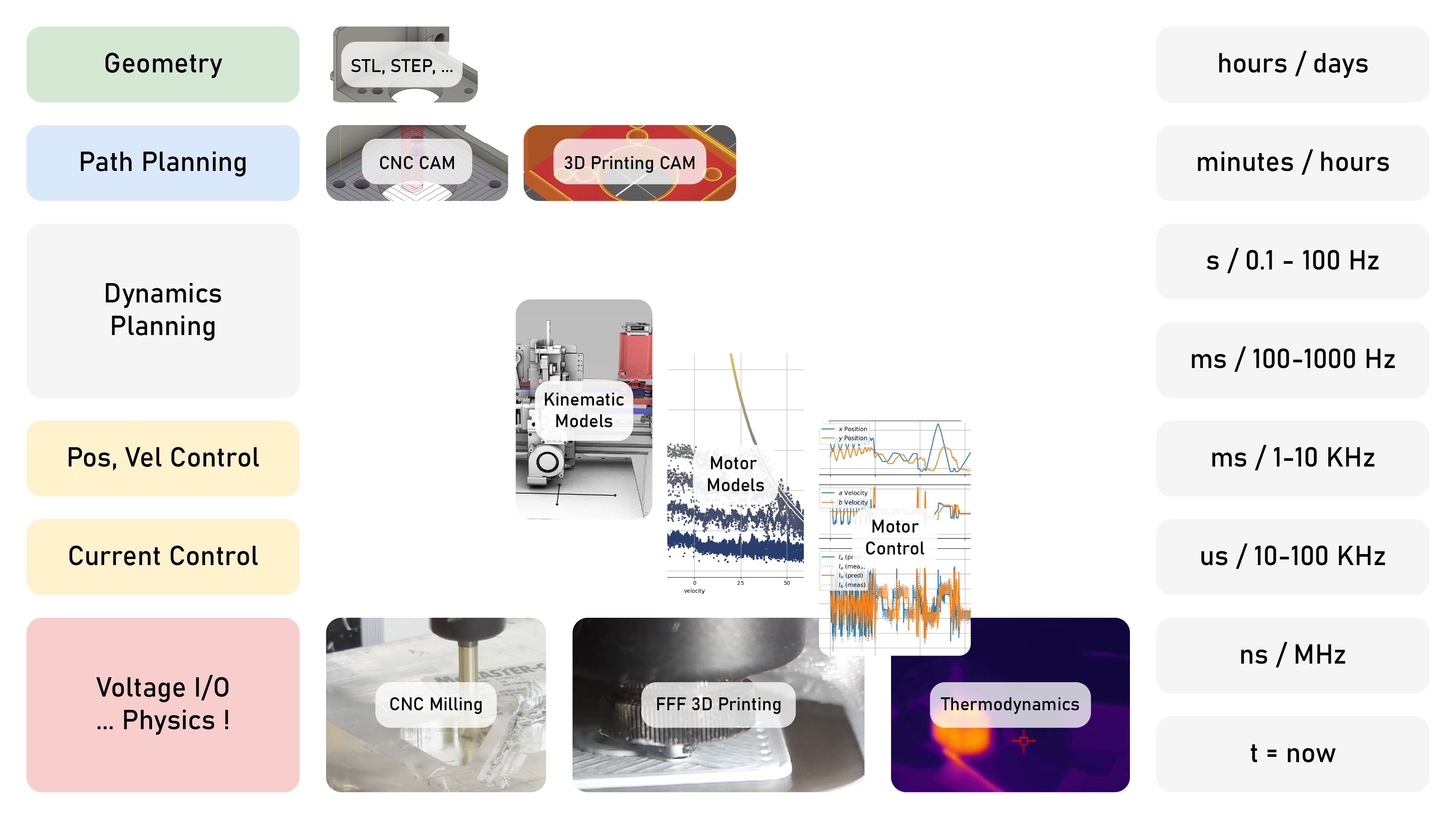
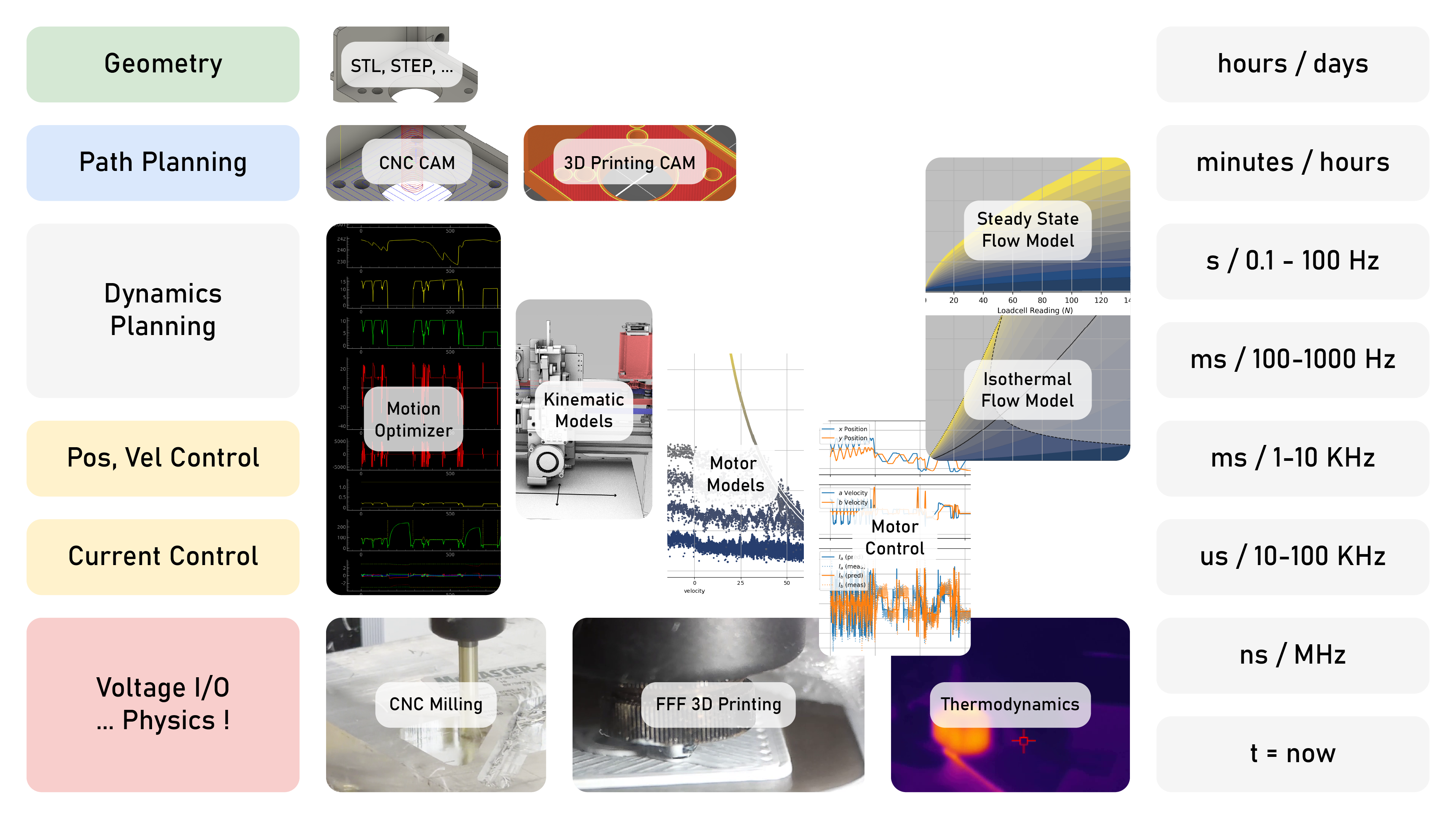
The End of GCode
Intelligent Modular Machines with Model Based Control
PhD Dissertation
Jake Robert Read
March 30th, 2026
MIT Center for Bits and Atoms
Cambridge, MA, United States
Neil Gershenfeld
Director, Center for Bits and Atoms
Massachusetts Institute of Technology
Director, Center for Bits and Atoms
Massachusetts Institute of Technology
Nadya Peek
Associate Professor, Human Centered Design and Engineering
University of Washington
Associate Professor, Human Centered Design and Engineering
University of Washington
Jon Seppala
Director, nSoft Consortium
National Institute of Standards and Technology
Director, nSoft Consortium
National Institute of Standards and Technology
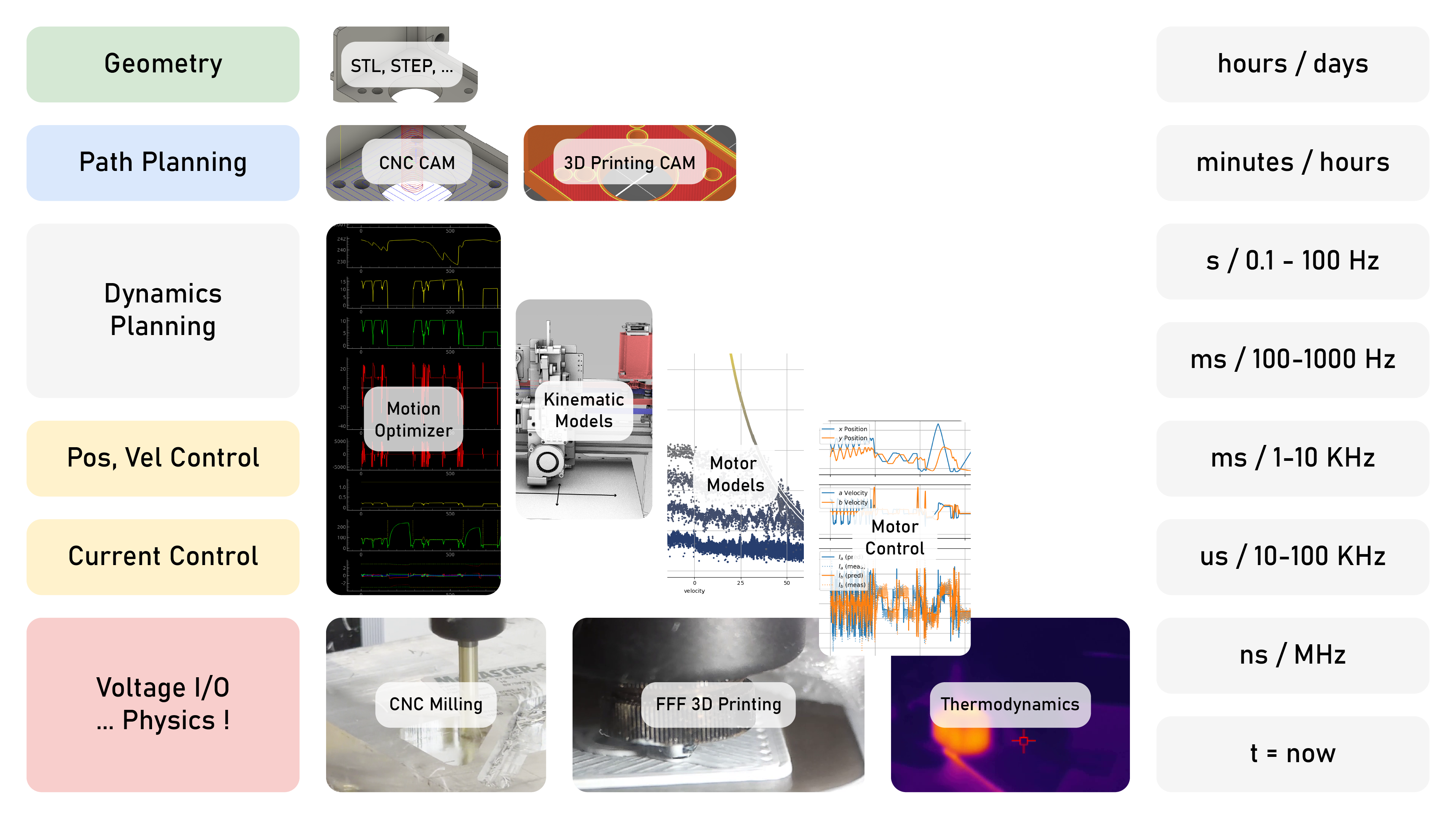
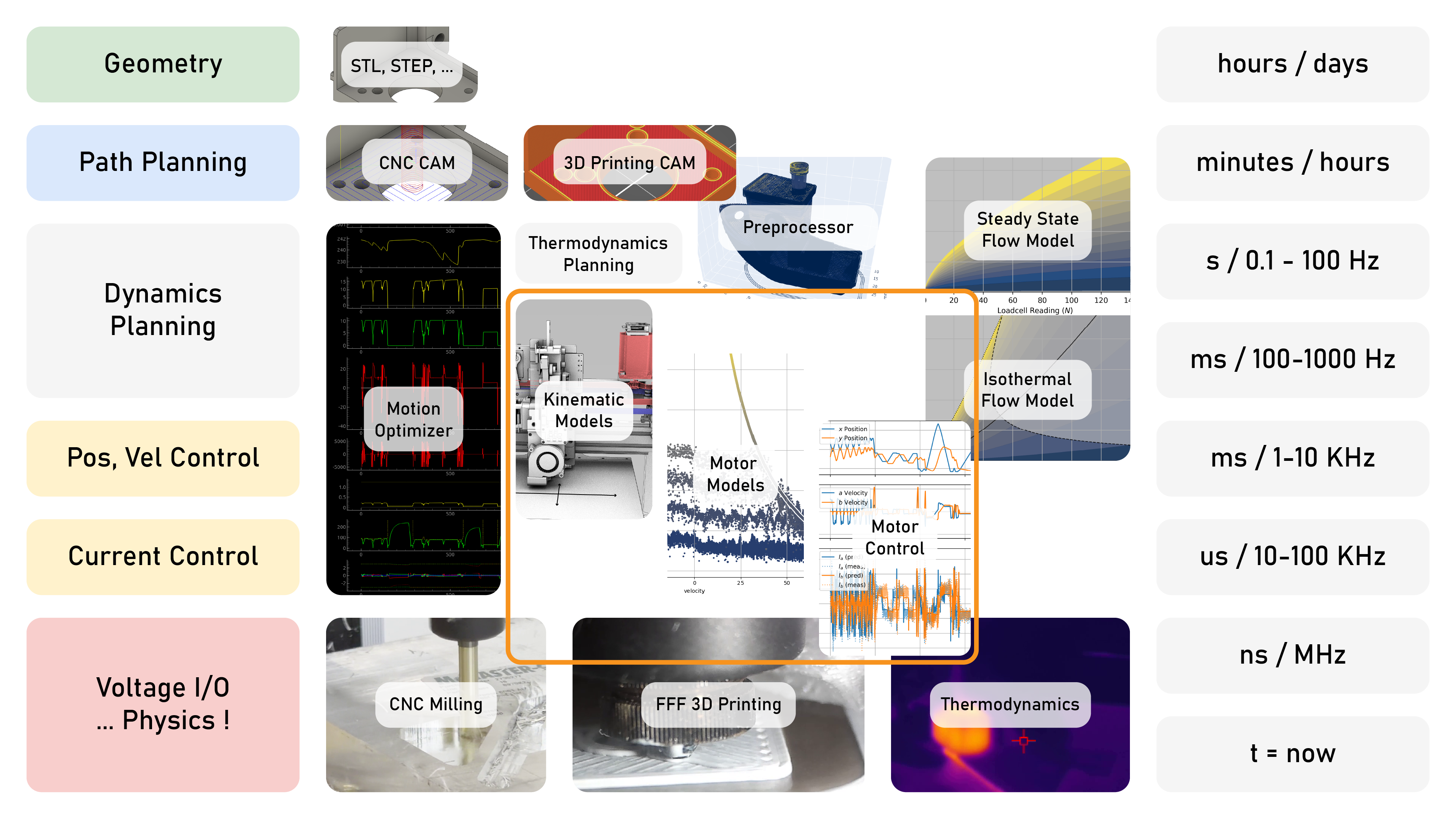
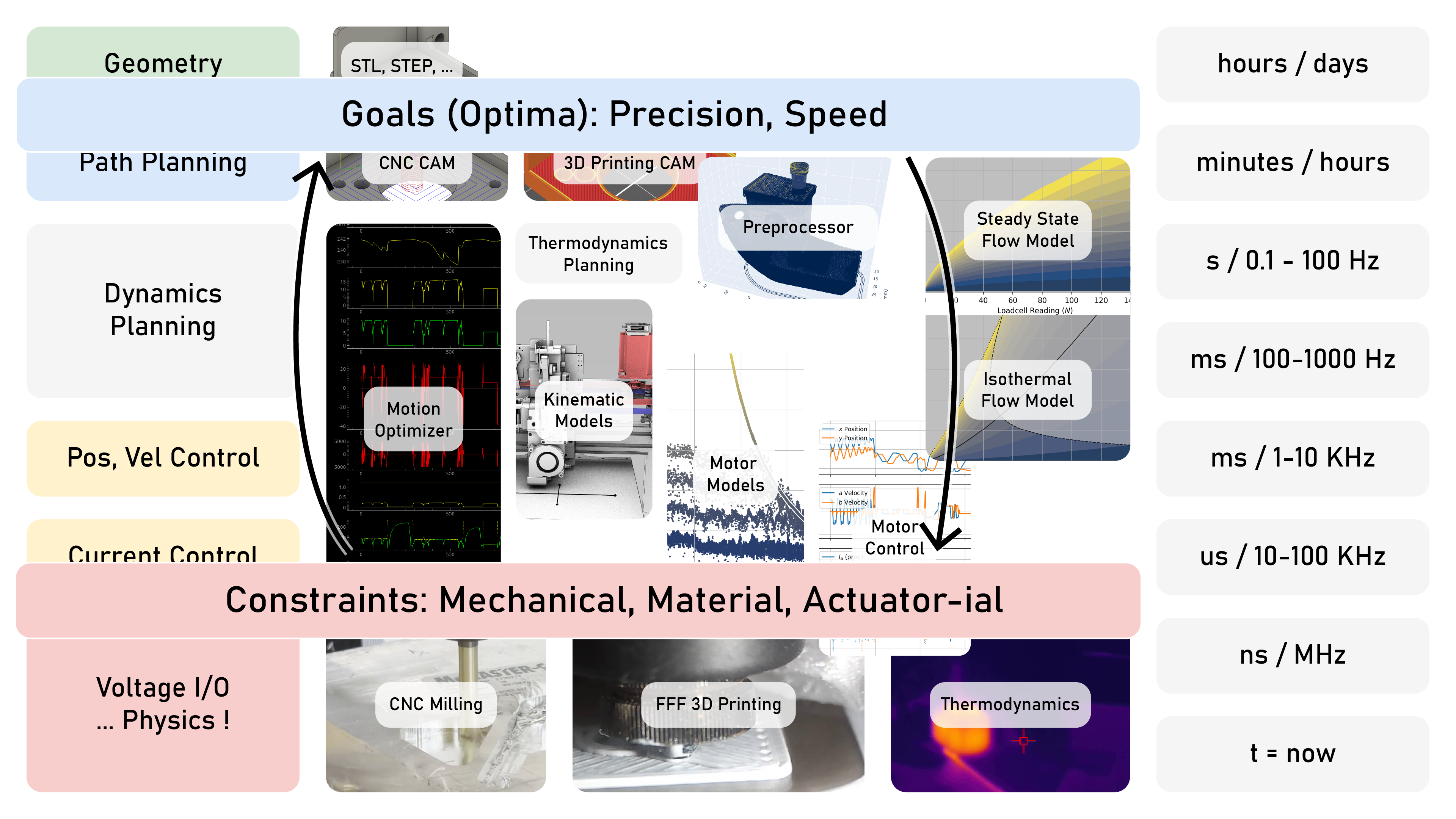
Can we make it easier to operate machines, without reducing human agency?
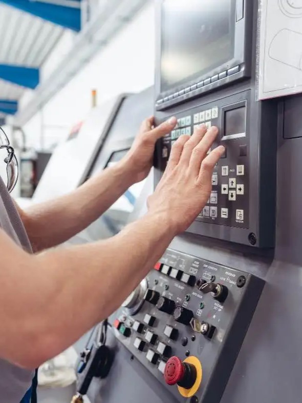
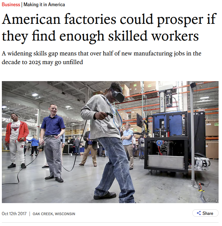
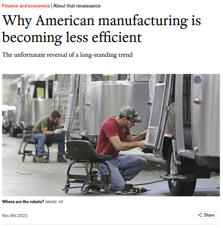
From The Economist
Nor can we improve those jobs' productivity; we aren't developing new automation rapidly
enough.
Famco 100 (1950's)
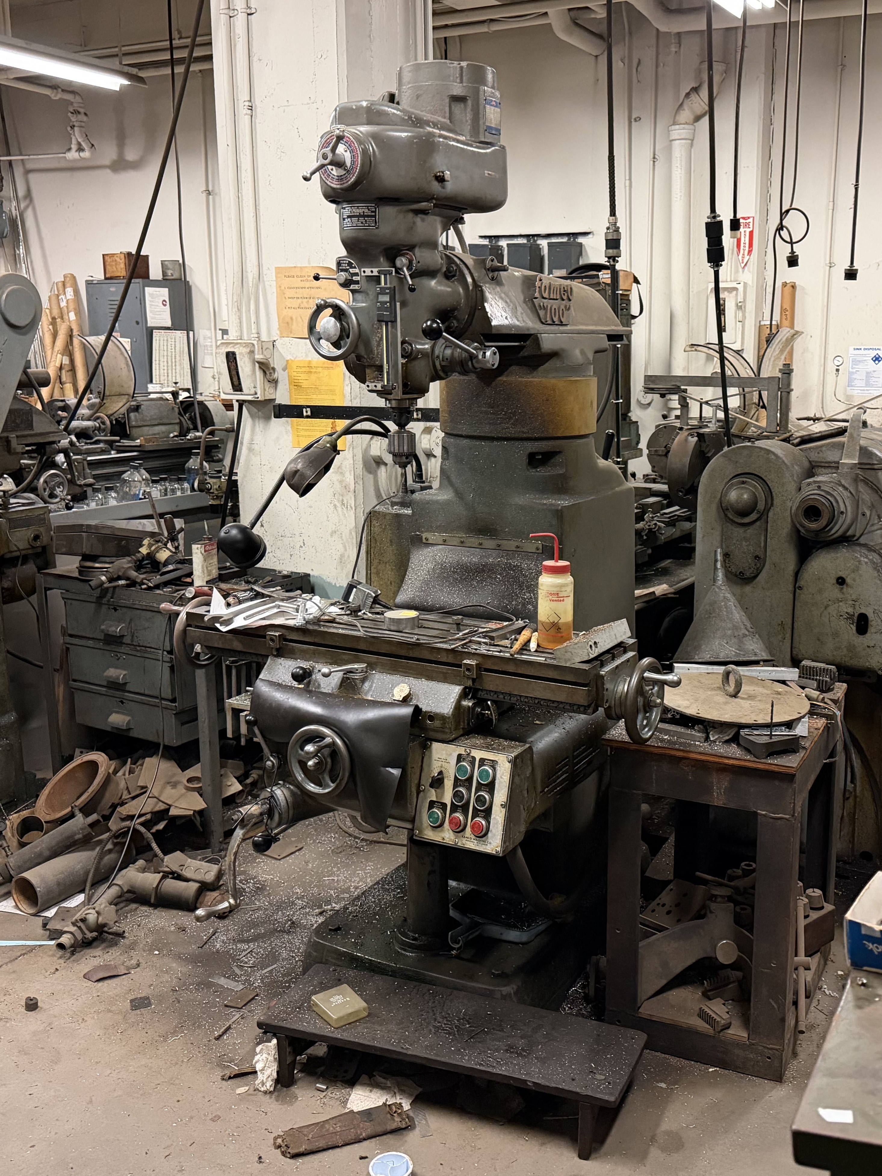
Can we imagine re-awakening old equipment with modular controllers?
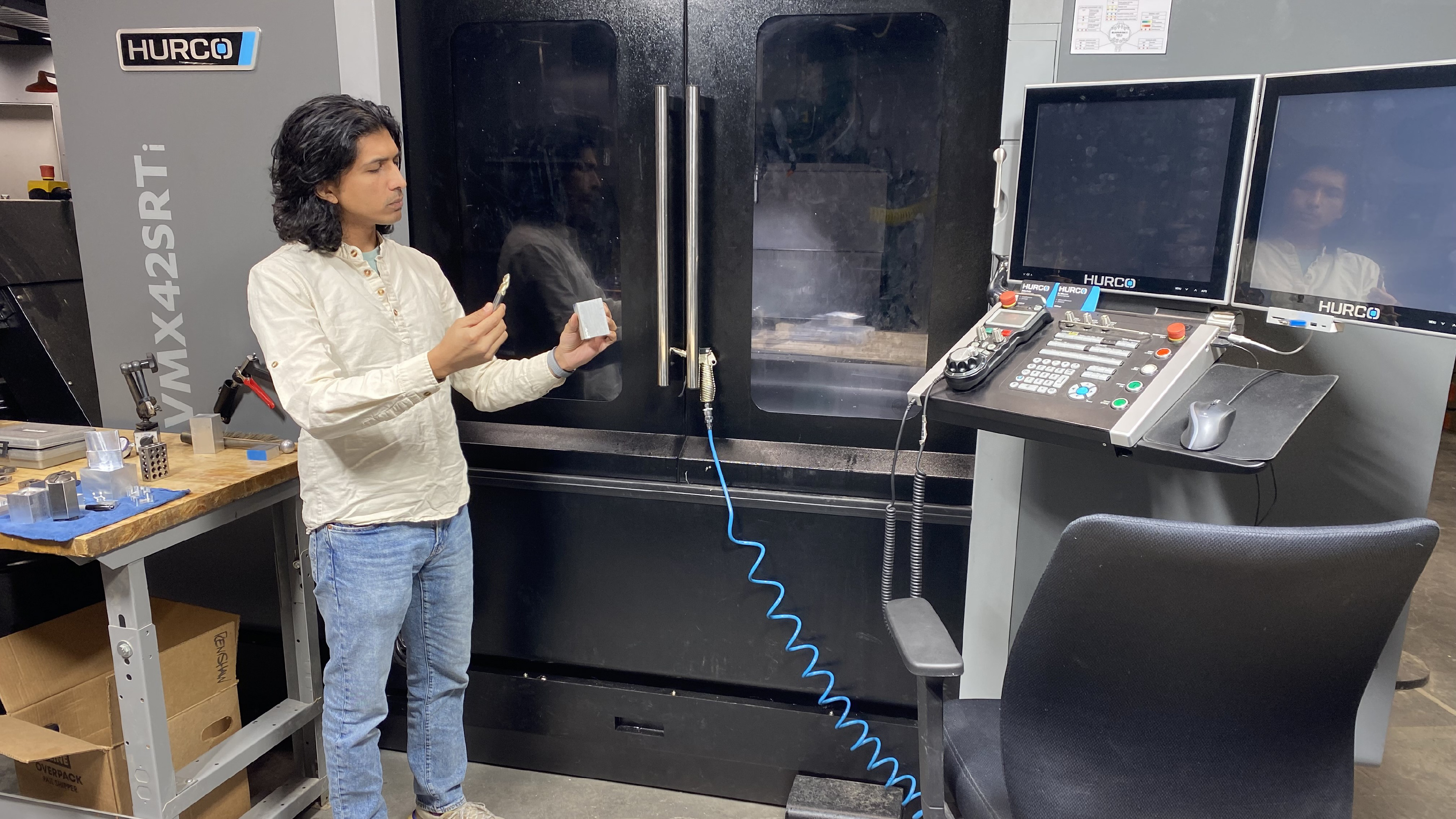
Hurco VMX42SRTi (2010's)
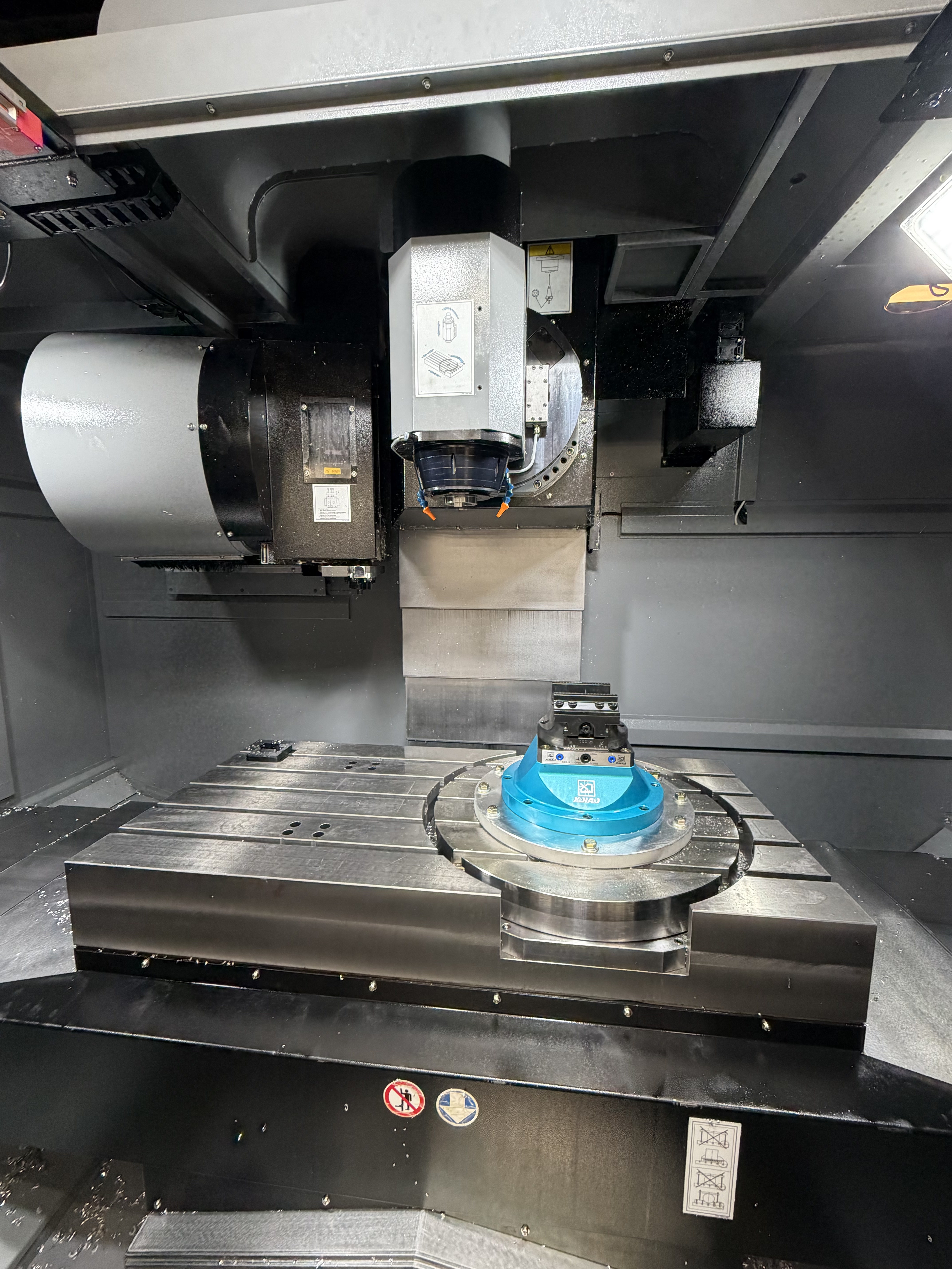
Can we make it easier to understand and develop machines?
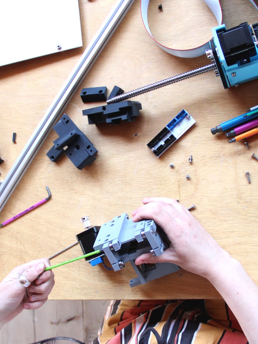
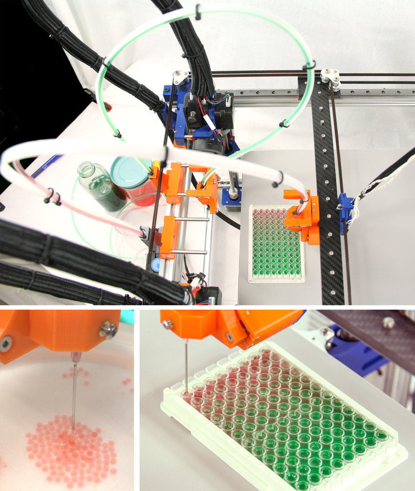
Vasquez, Joshua, et al. "Jubilee Demo: An Extensible Machine for Multi-Tool Fabrication."
Extended Abstracts of the 2020 CHI Conference on Human Factors in Computing Systems. 2020.
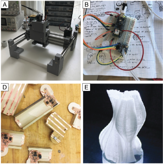
Peek, Nadya, et al. "Making at a distance: teaching hands-on courses during the pandemic."
Extended Abstracts of the 2021 CHI Conference on Human Factors in Computing Systems. 2021.
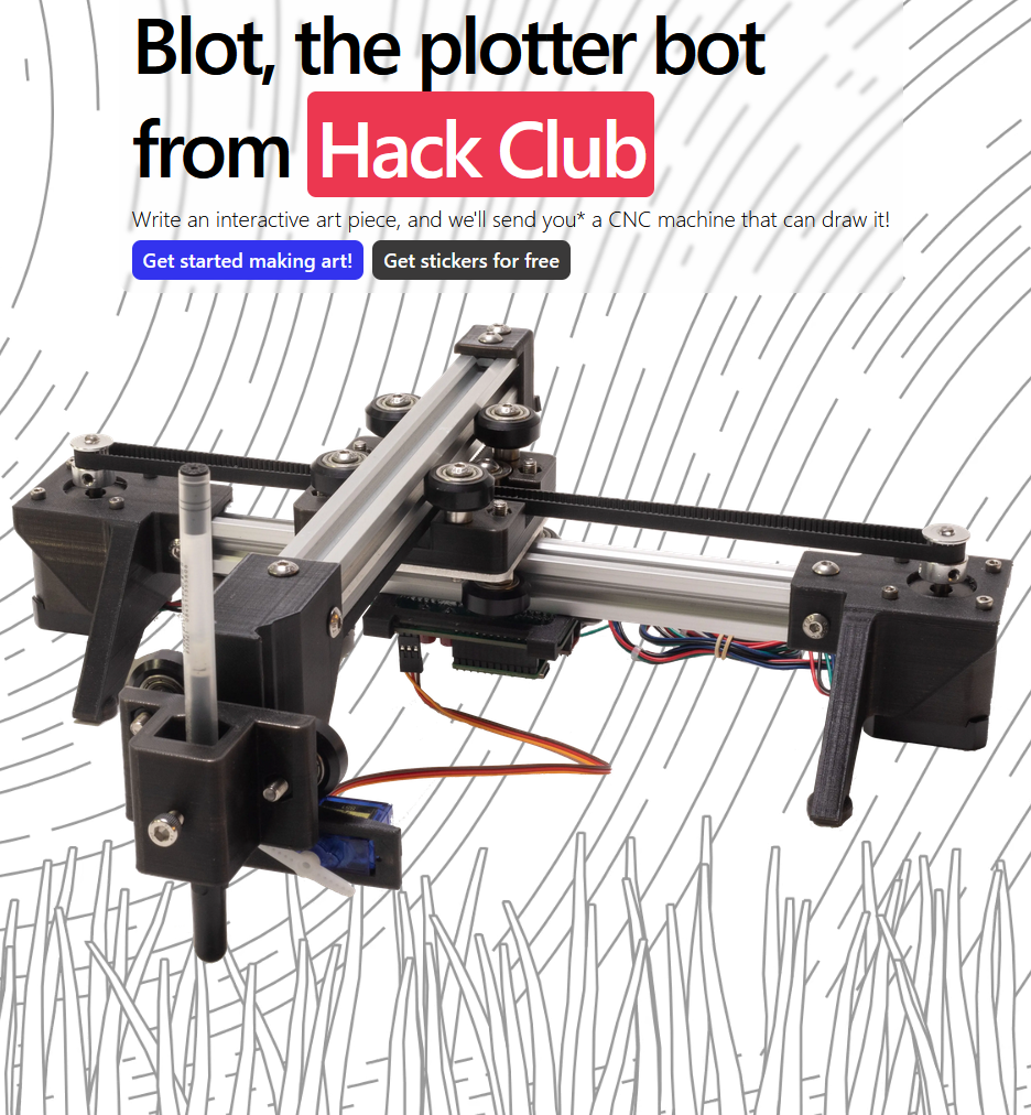
Hack Club and Leo McElroy
https://blot.hackclub.com/
https://blot.hackclub.com/
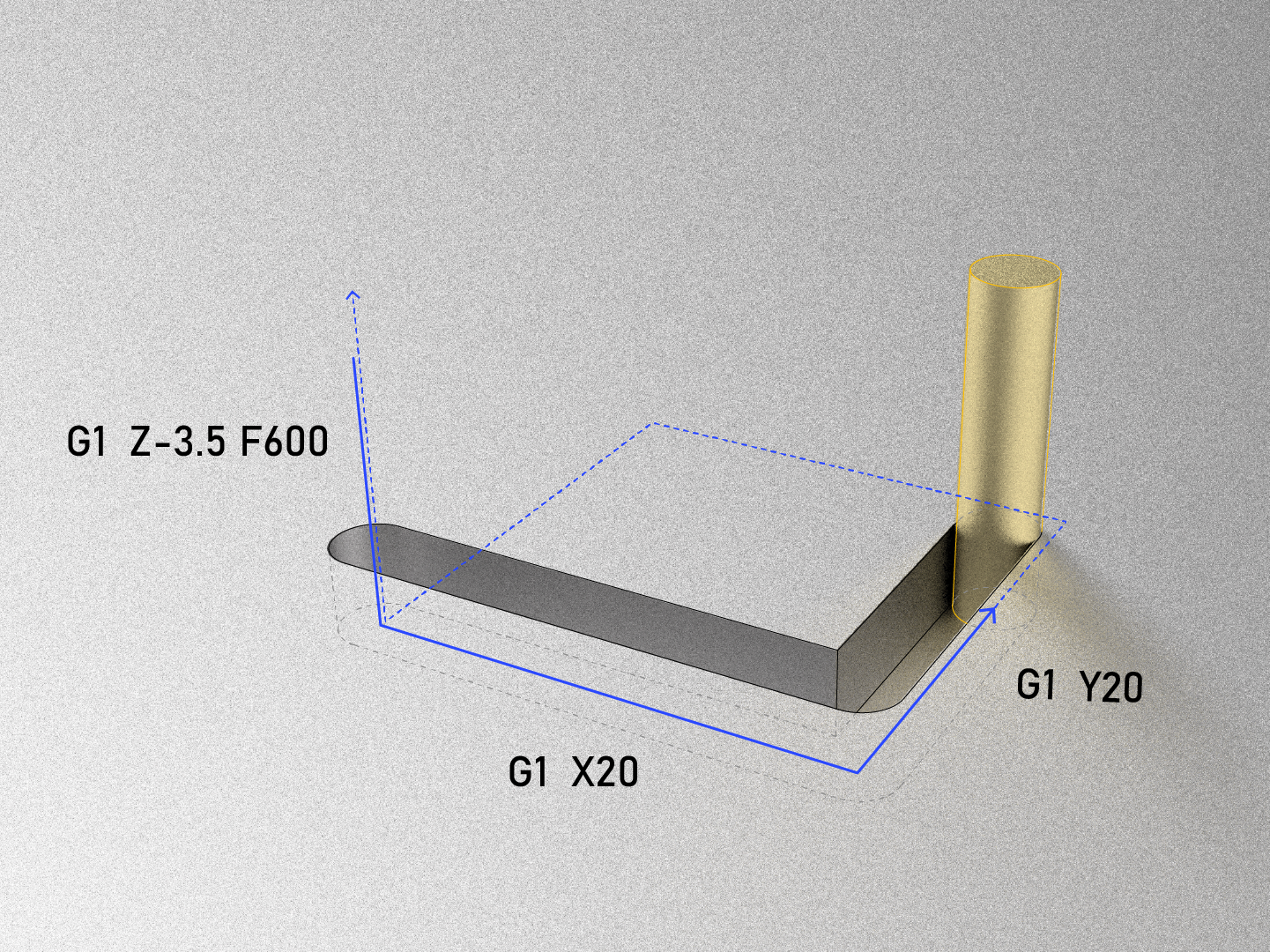
G21                   ; use millimeters
G28                   ; run the homing routine
G92 X110 Y120 Z30     ; set current position to (110, 120, 30)
G0  X10 Y10 Z10 F6000 ; "rapid" in *units per minute*
M3  S5000             ; turn the spindle on, at 5000 RPM
G1  Z-3.5 F600        ; plunge from (10, 10, 10) to (10, 10, -3.5)
G1  X20               ; draw a square, go to the right,
G1  Y20               ; go backwards 10mm
G1  X10               ; go to the left 10mm
G1  Y10               ; go forwards 10mm
G1  Z10               ; go up to Z10, exiting the material
M5                    ; stop the spindle
G0  X110 Y120 Z30     ; return to the position after homing (at 6000)
A simple GCode program, for a milling machine.
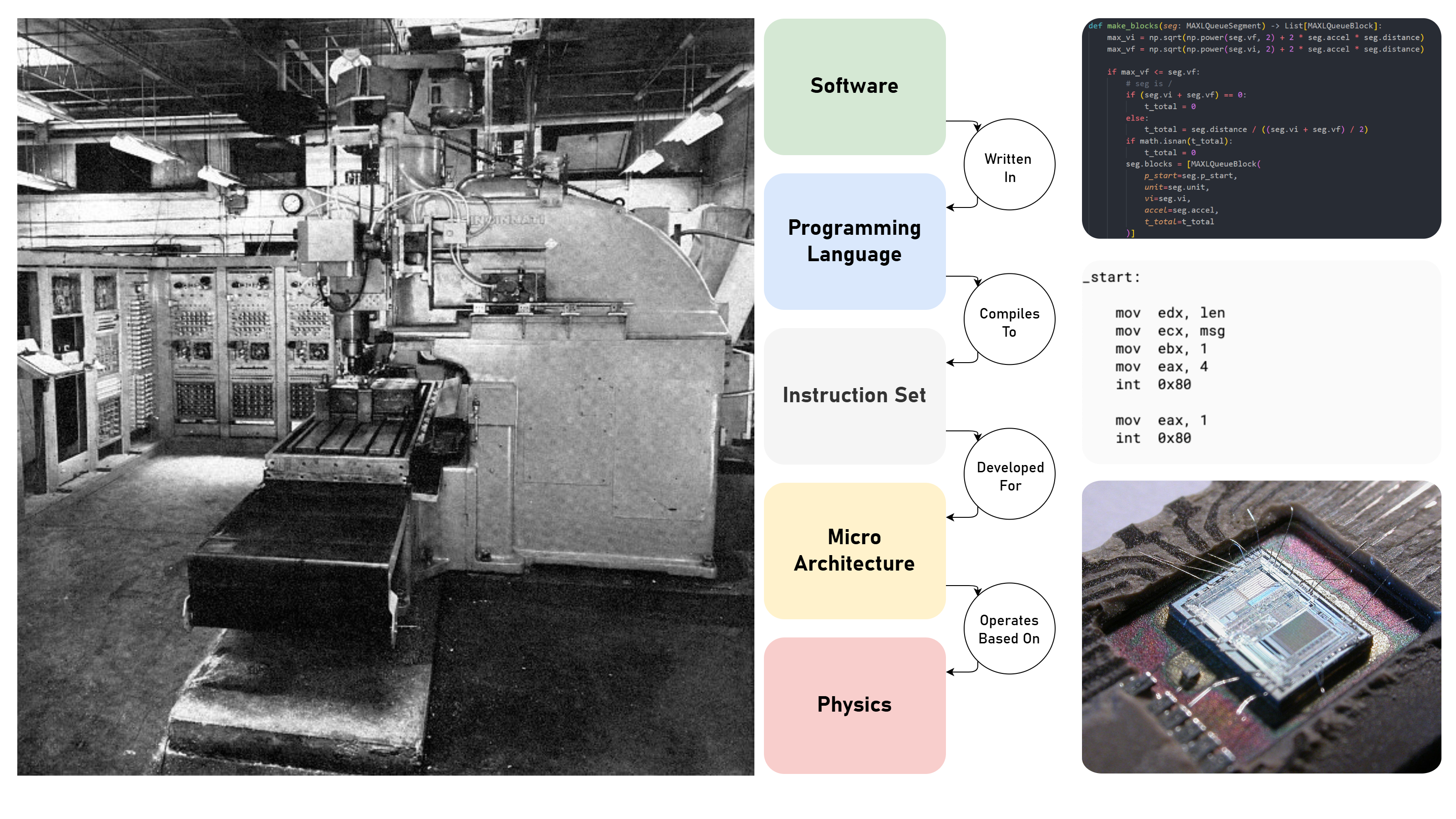
GCode was invented alongside the first CNC machine, in a milieu of computer scientists who were
developing top-down, feed-forward design patterns for system abstraction.
Noble, David. Forces of production: A social history of industrial automation. Routledge, 2017.
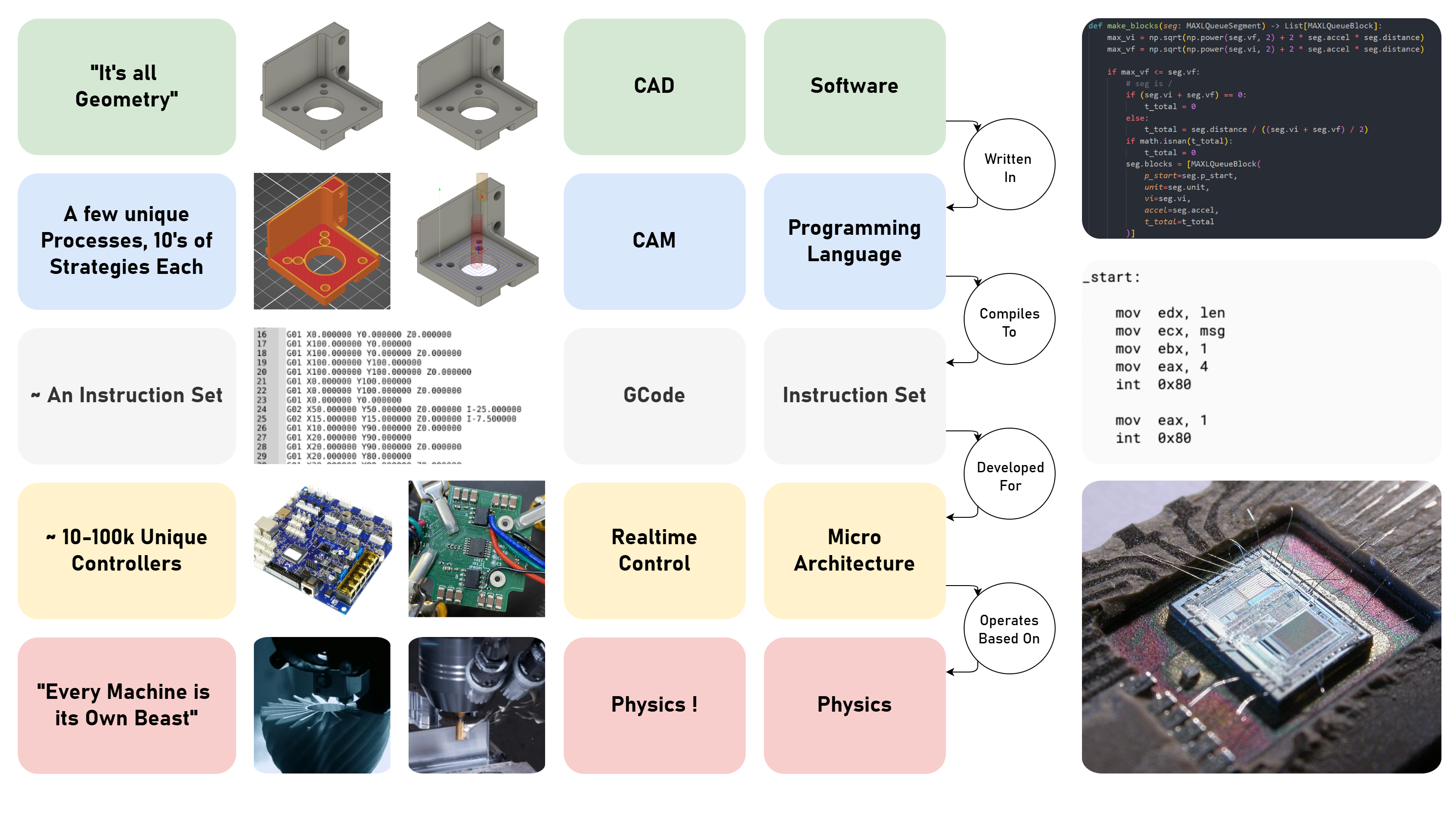
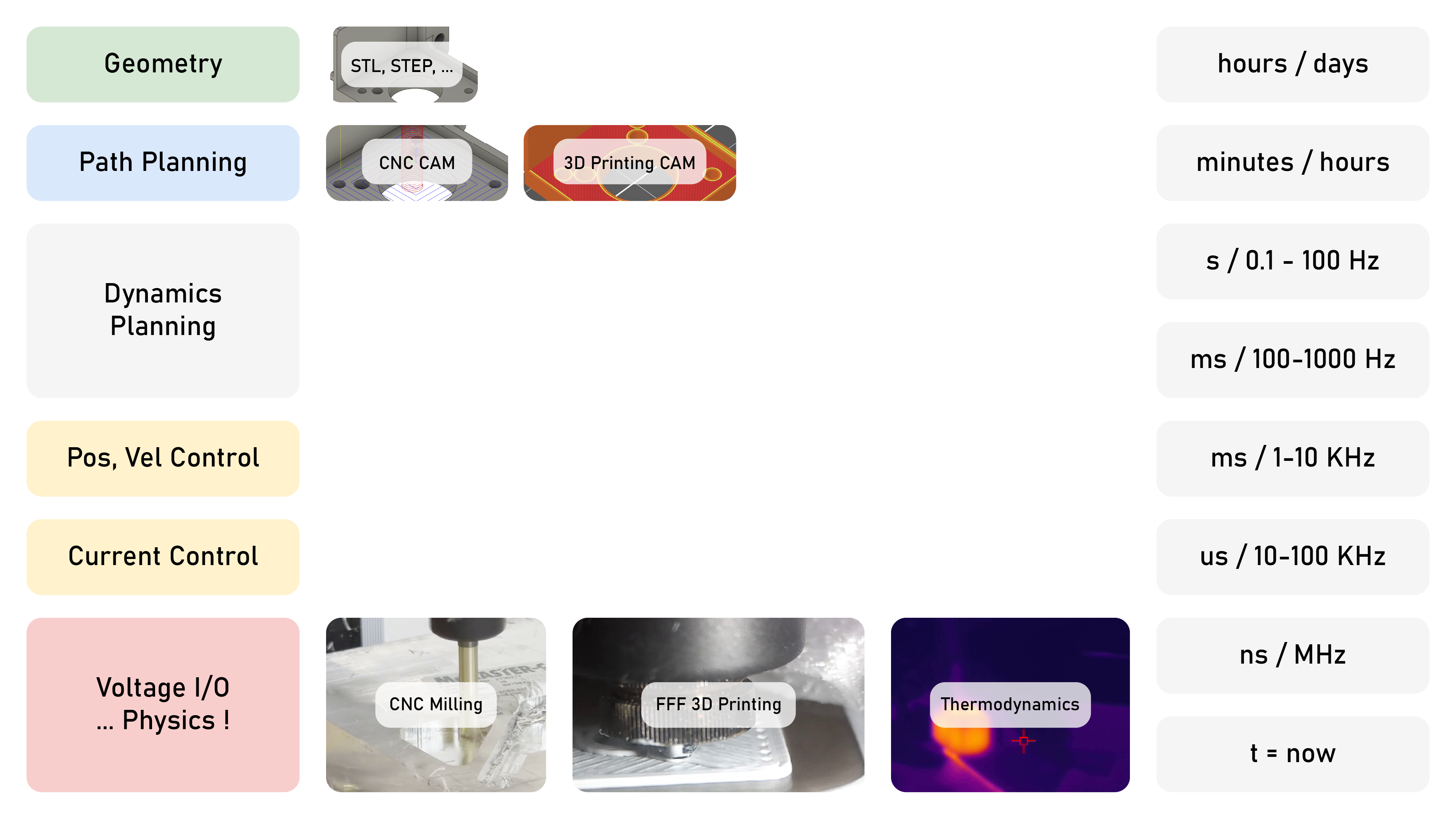
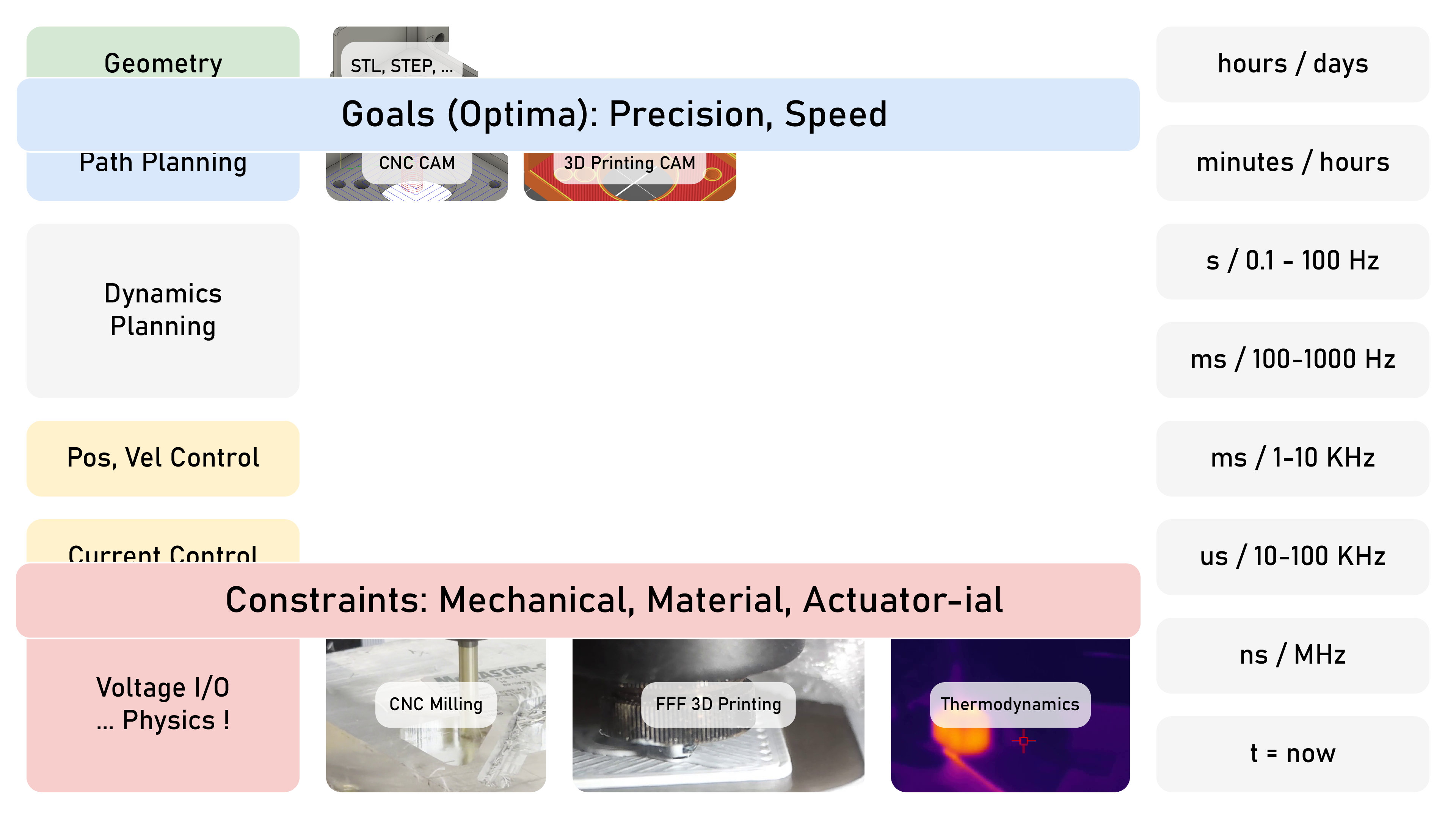
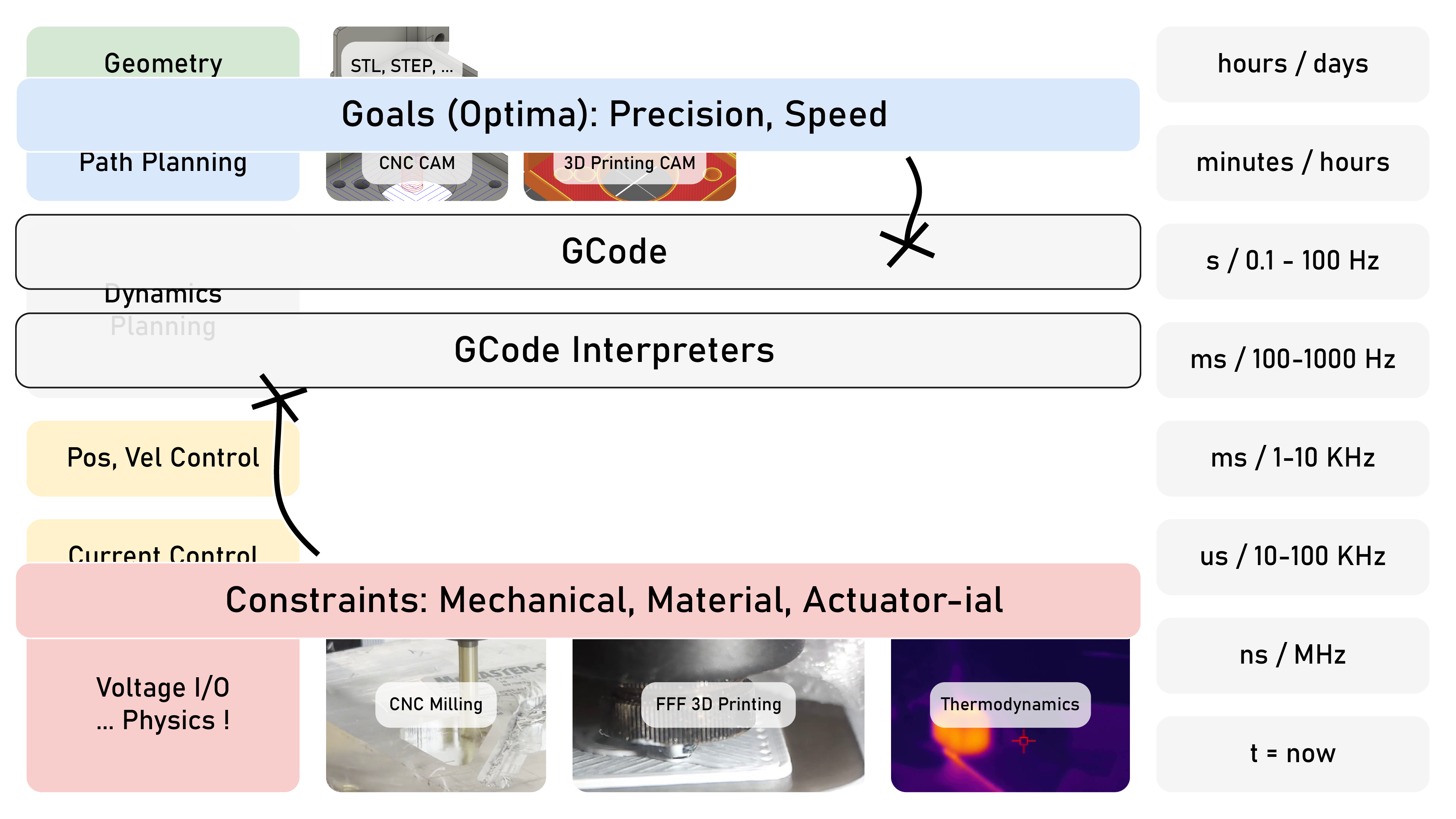
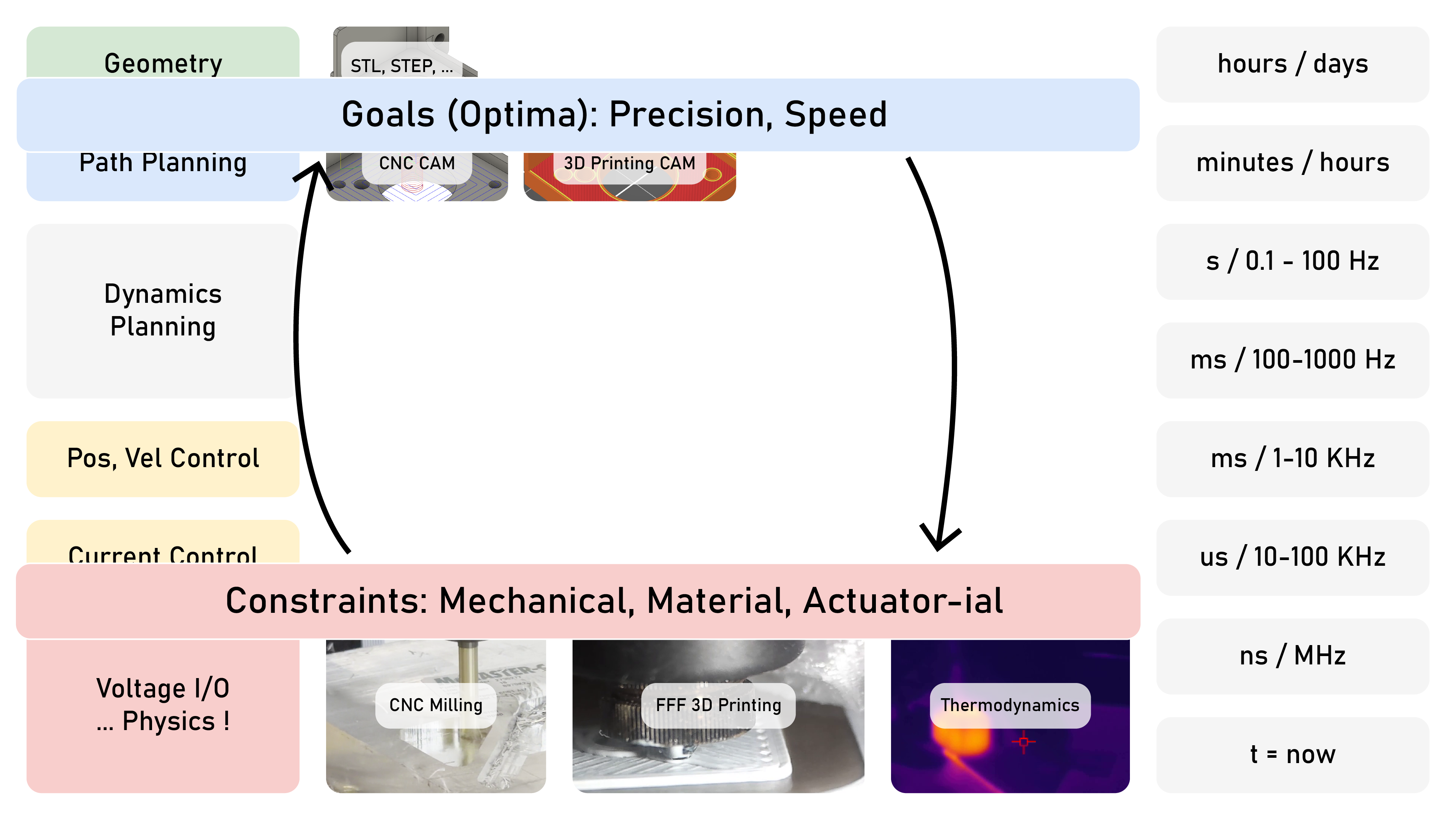
If machine control is a constrained optimization task, can we make that explicit?
Does machine performance improve if we do?
Does machine performance improve if we do?
Can we use machine models to describe those constraints?
What types of models would enable this?
What can we learn from those models - as machine designers and users?
What types of models would enable this?
What can we learn from those models - as machine designers and users?
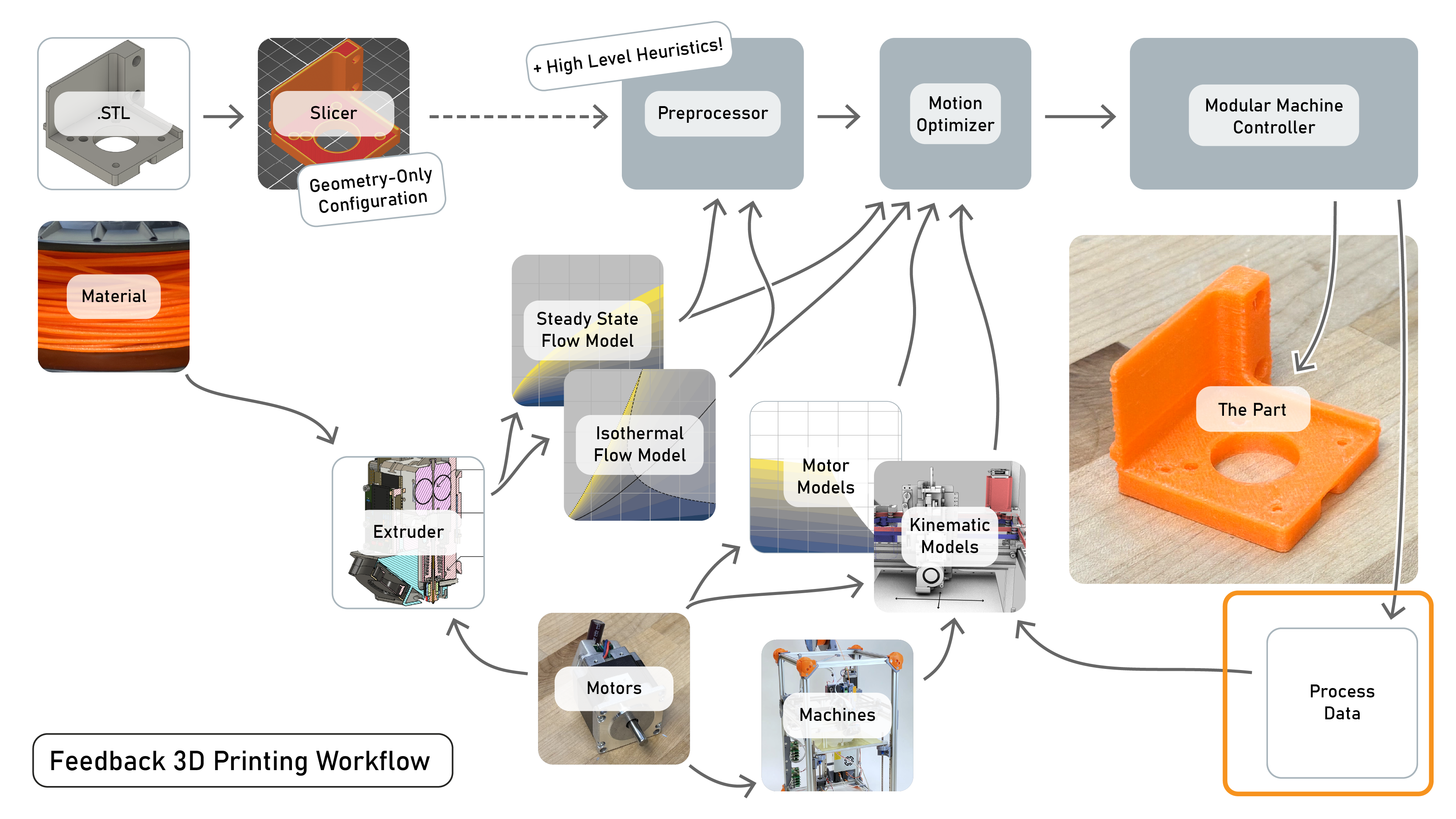
Can we frame entire workflows as model-based optimizations?
How can we leave room for heuristics, where models fail to capture details?
How can we leave room for heuristics, where models fail to capture details?
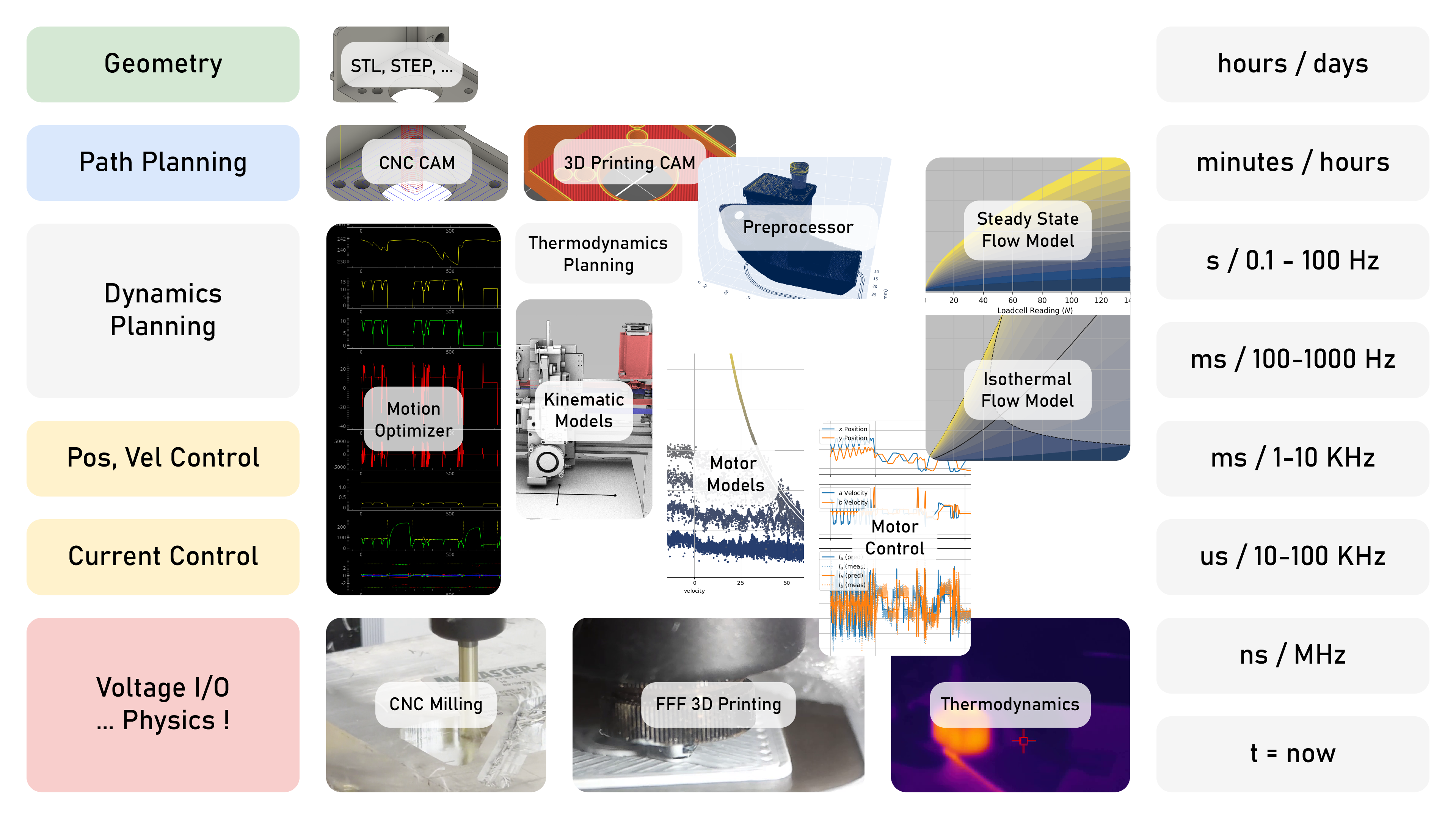
What kind of systems architecture would enable all of this?
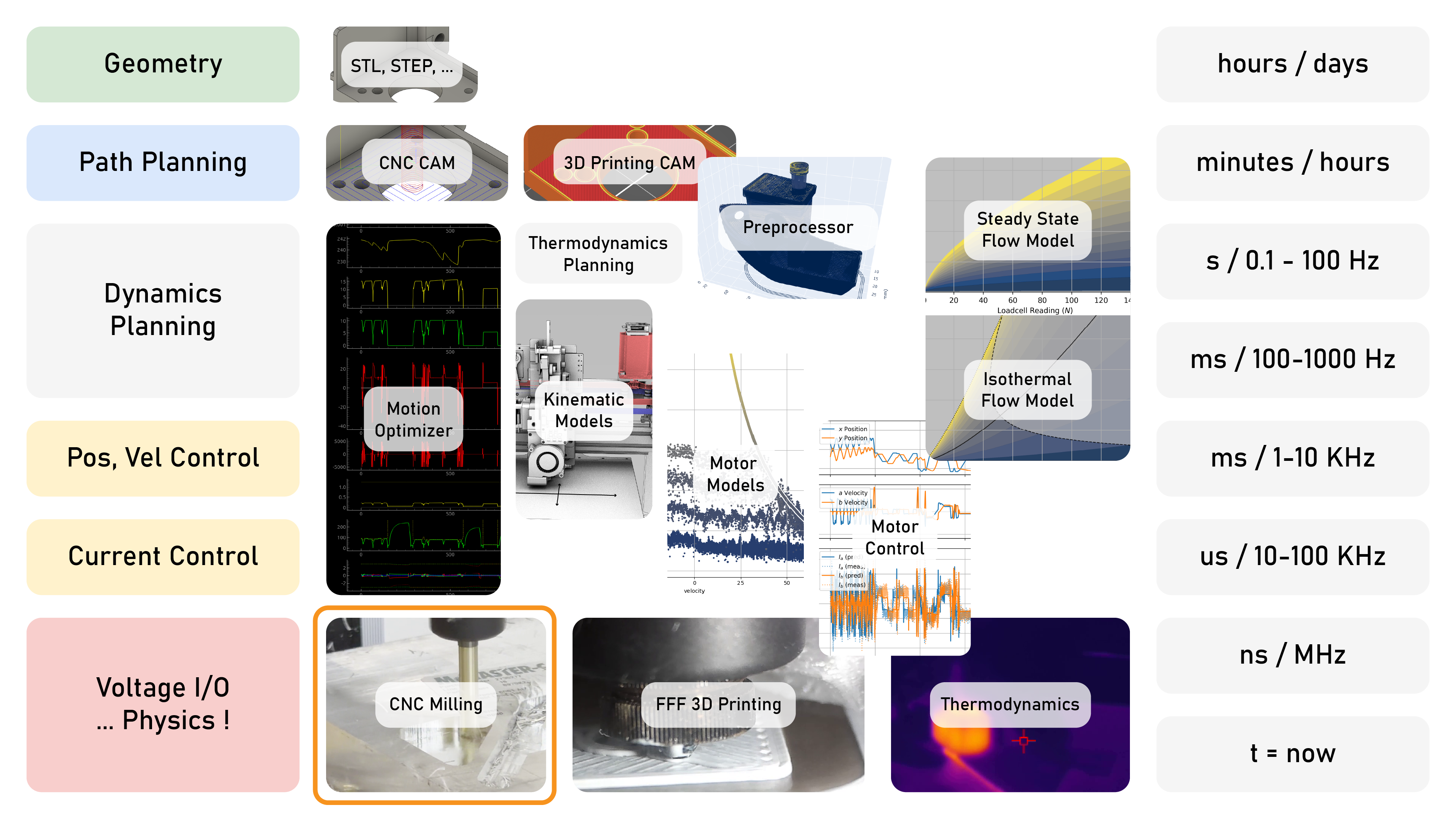
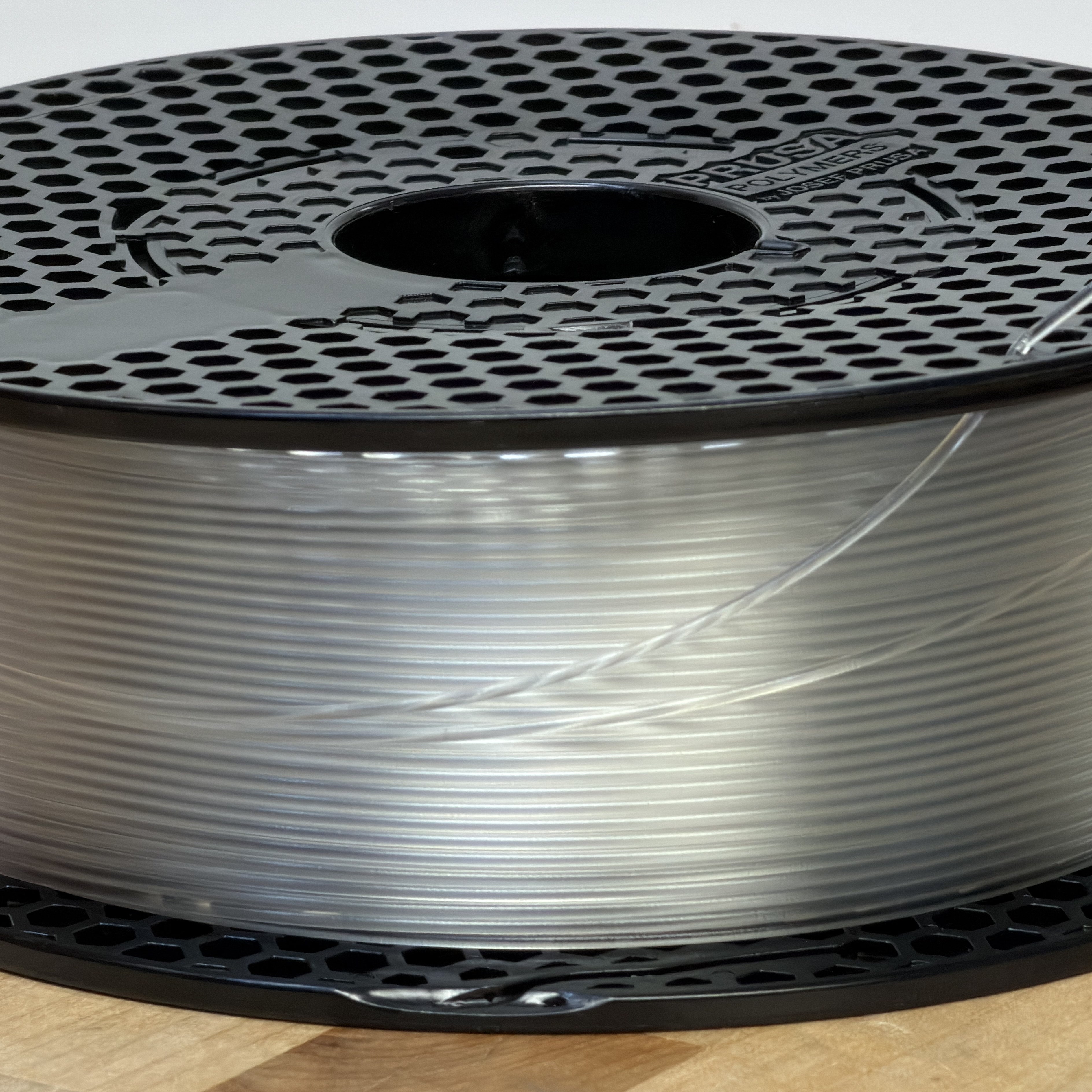
From Formation Plastics.
Built Up Edge (BUE) Formation, via YouTube.
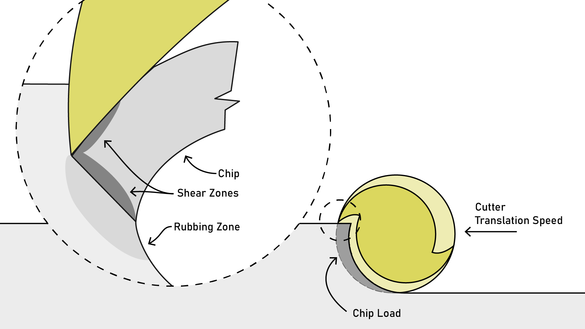
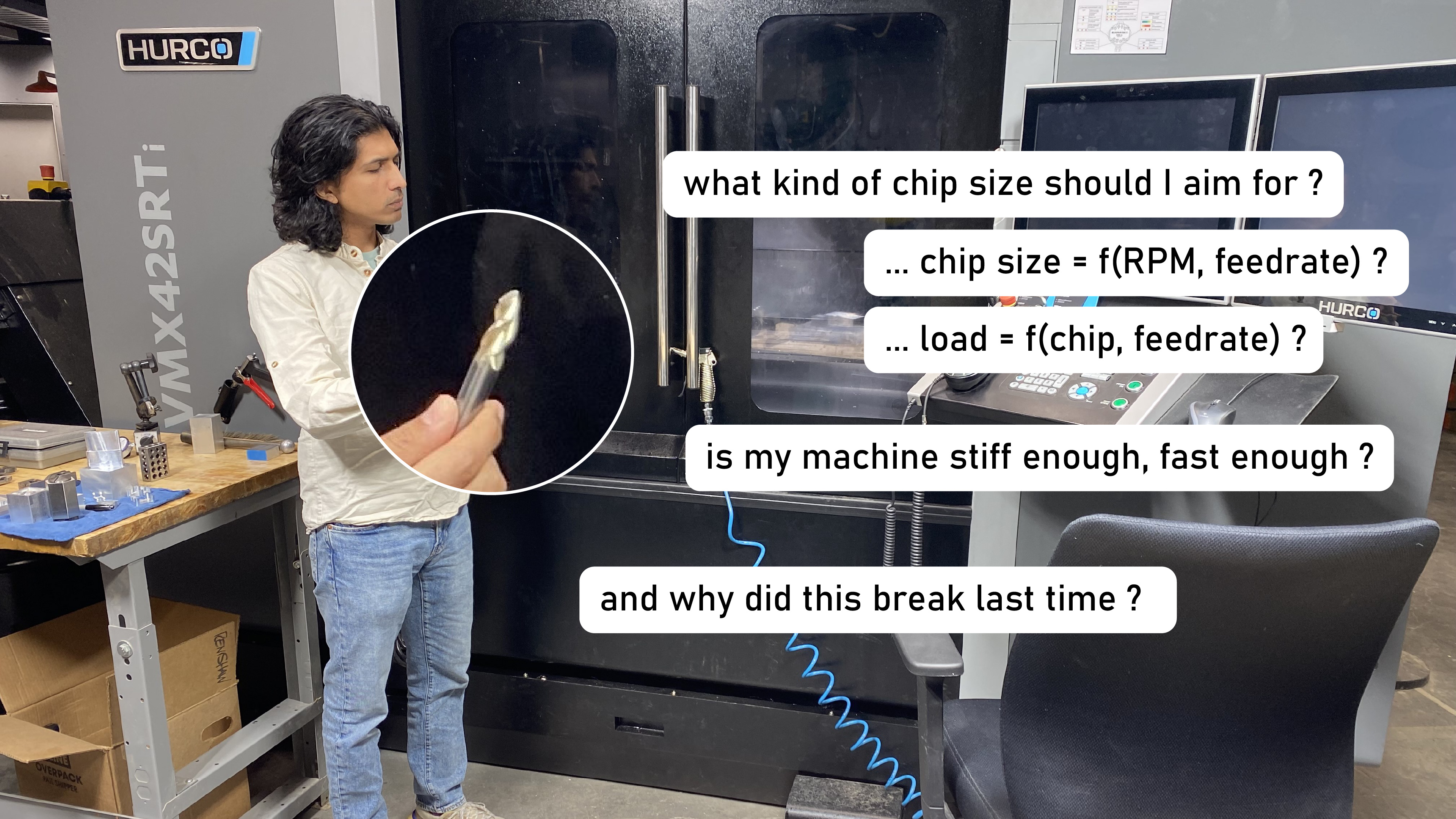
CNC machining physics: the tool has a number of cutting edges (flutes),
that cut chips.
The size of the chip, aka chip load, is a function of the tool's RPM and the machine's speed.
The size of the chip, aka chip load, is a function of the tool's RPM and the machine's speed.
Maintaining chip load is important: if the machine slows down
too much, we risk rubbing instead of cutting.
Schmitz, Tony L, and K Scott Smith. 2009. “Machining Dynamics.” Springer.
CNC programming involves picking feeds (cut sizes)
and speeds (for motion, and spindle RPM).
As well as strategies; how tool paths will be planned.
and speeds (for motion, and spindle RPM).
As well as strategies; how tool paths will be planned.
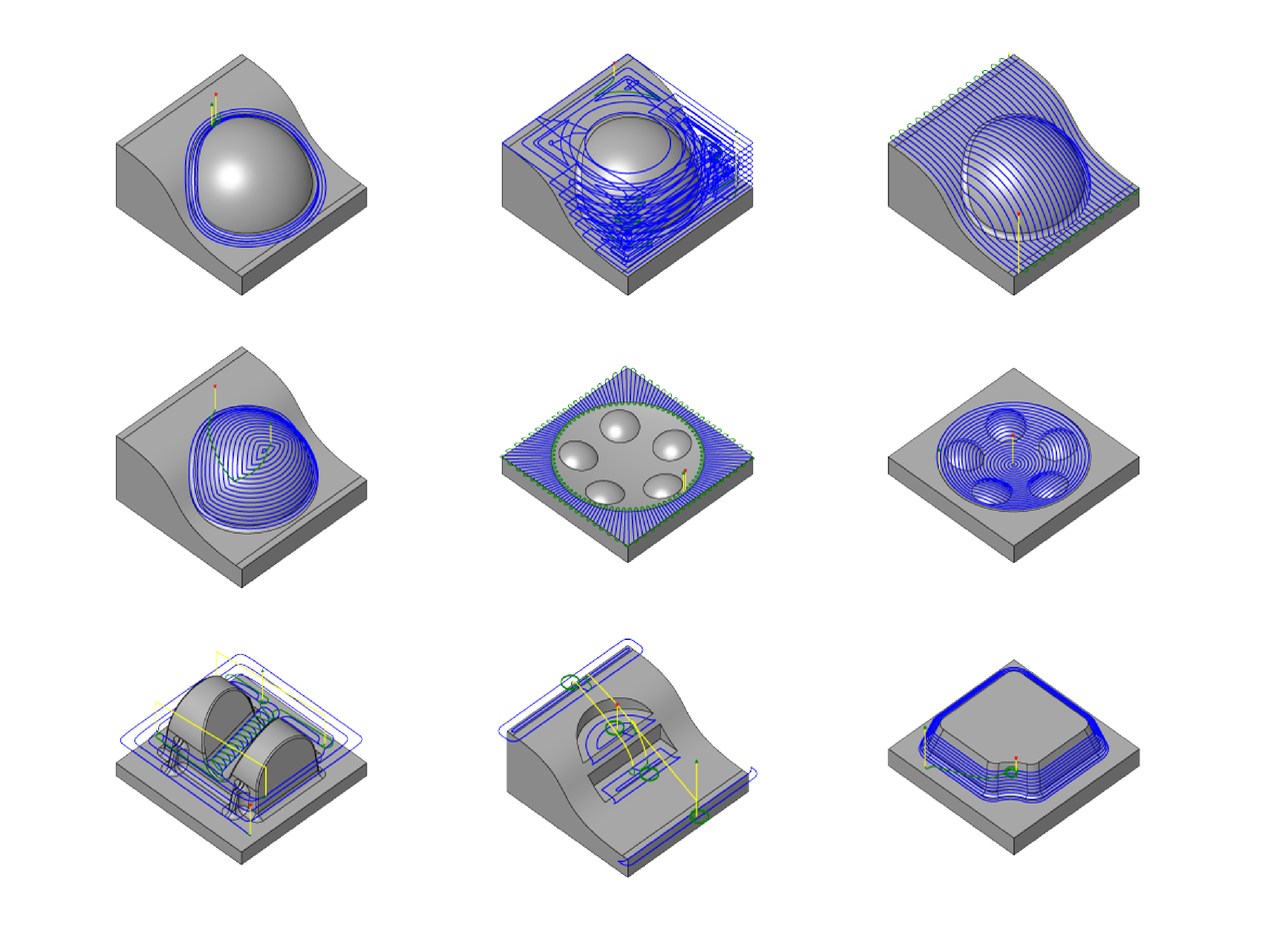
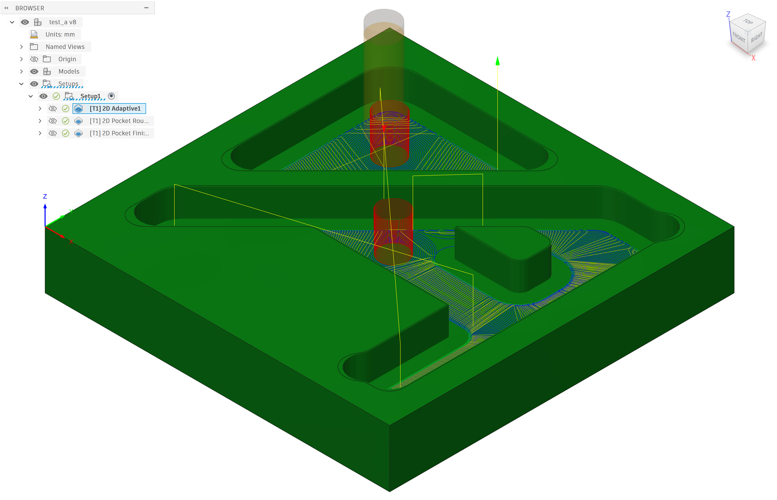
Milling Strategies via
AutoDesk Fusion
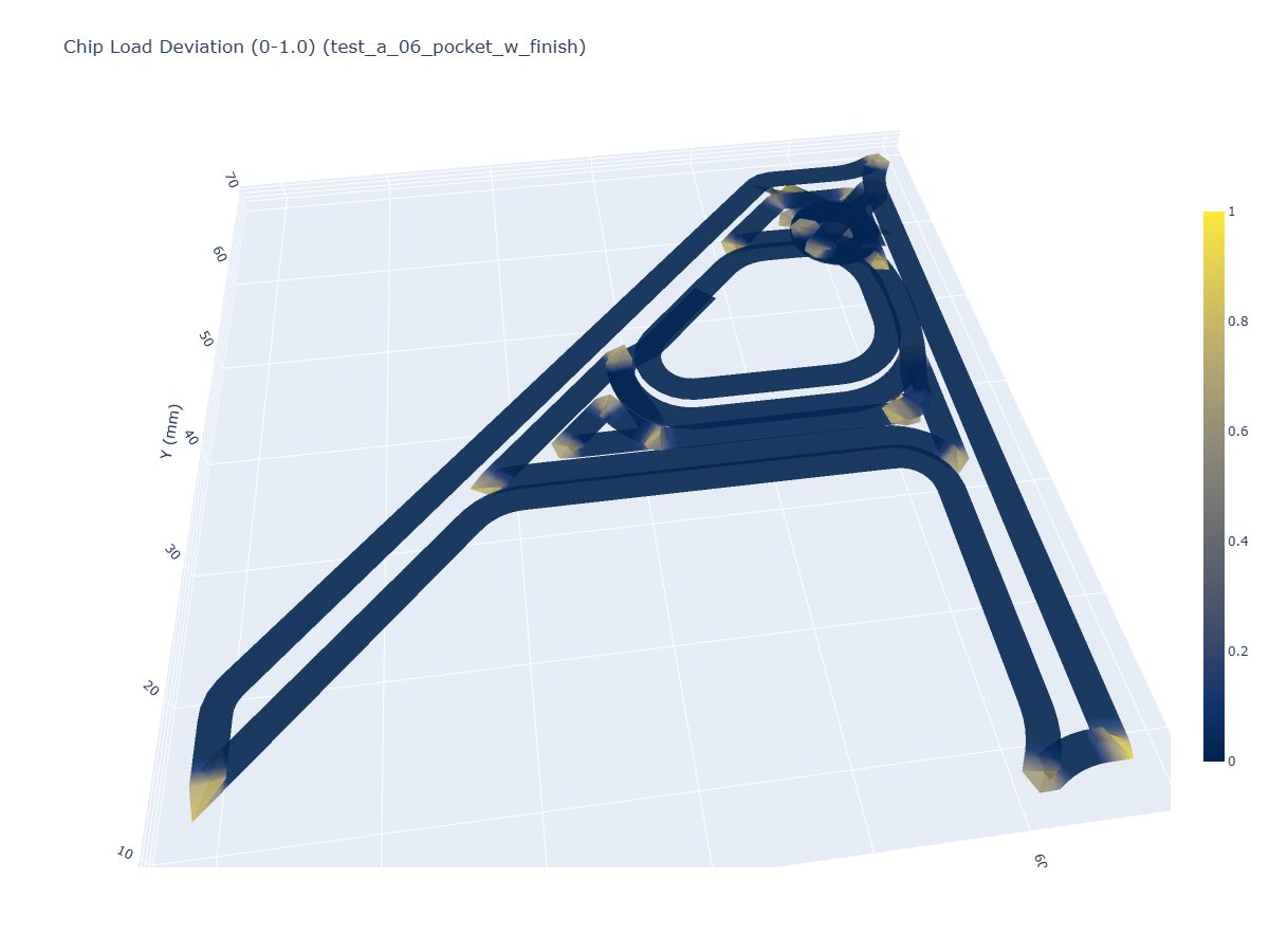
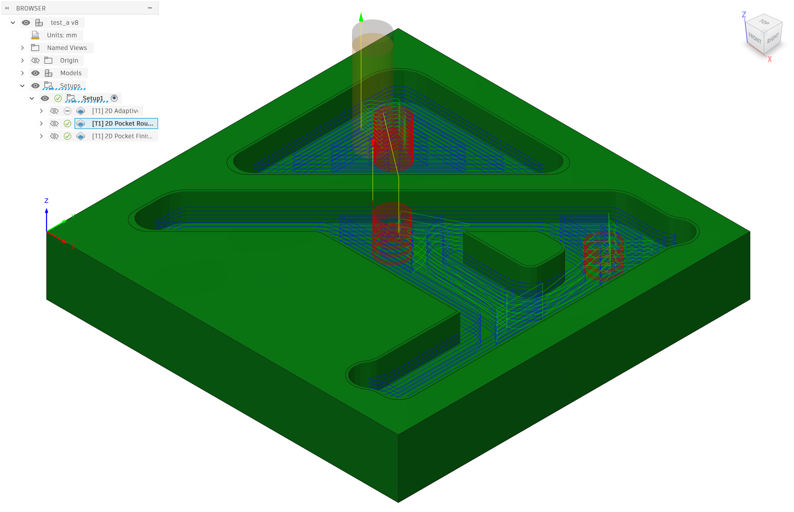
A 2D Pocket Toolpath (bottom) and chip load deviations (top).
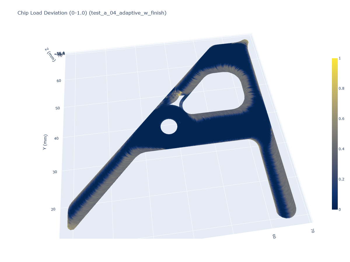
An Adaptive Toolpath (bottom) and chip load deviations (top).
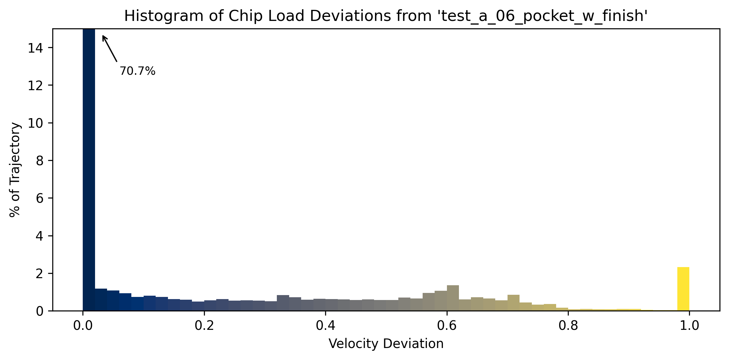
Pocket Toolpath w/ 3D deviations and histogram.
(blue good, yellow bad).
(blue good, yellow bad).
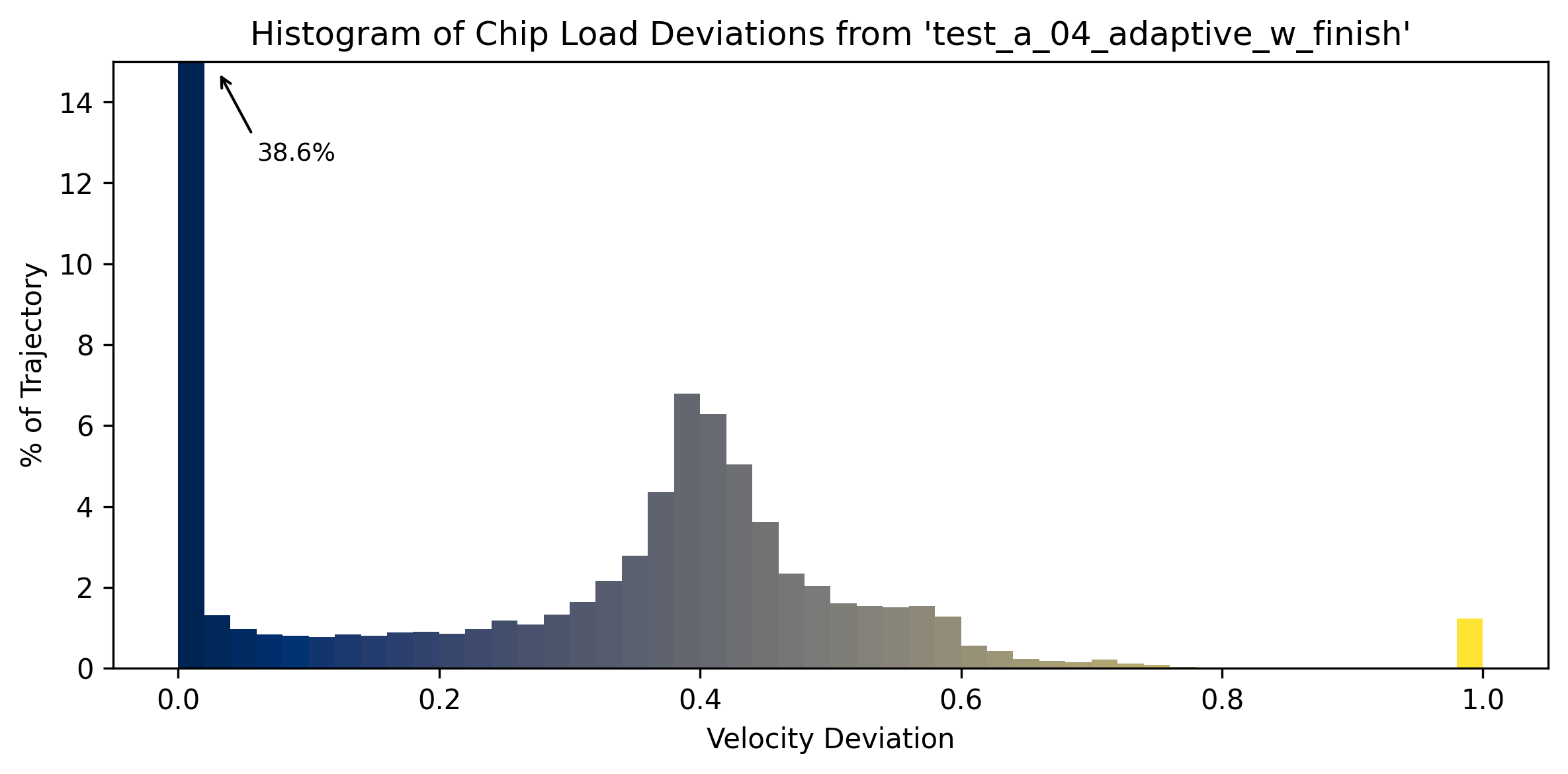
Adaptive Toolpath w/ 3D deviations and histogram.
(blue good, yellow bad).
(blue good, yellow bad).
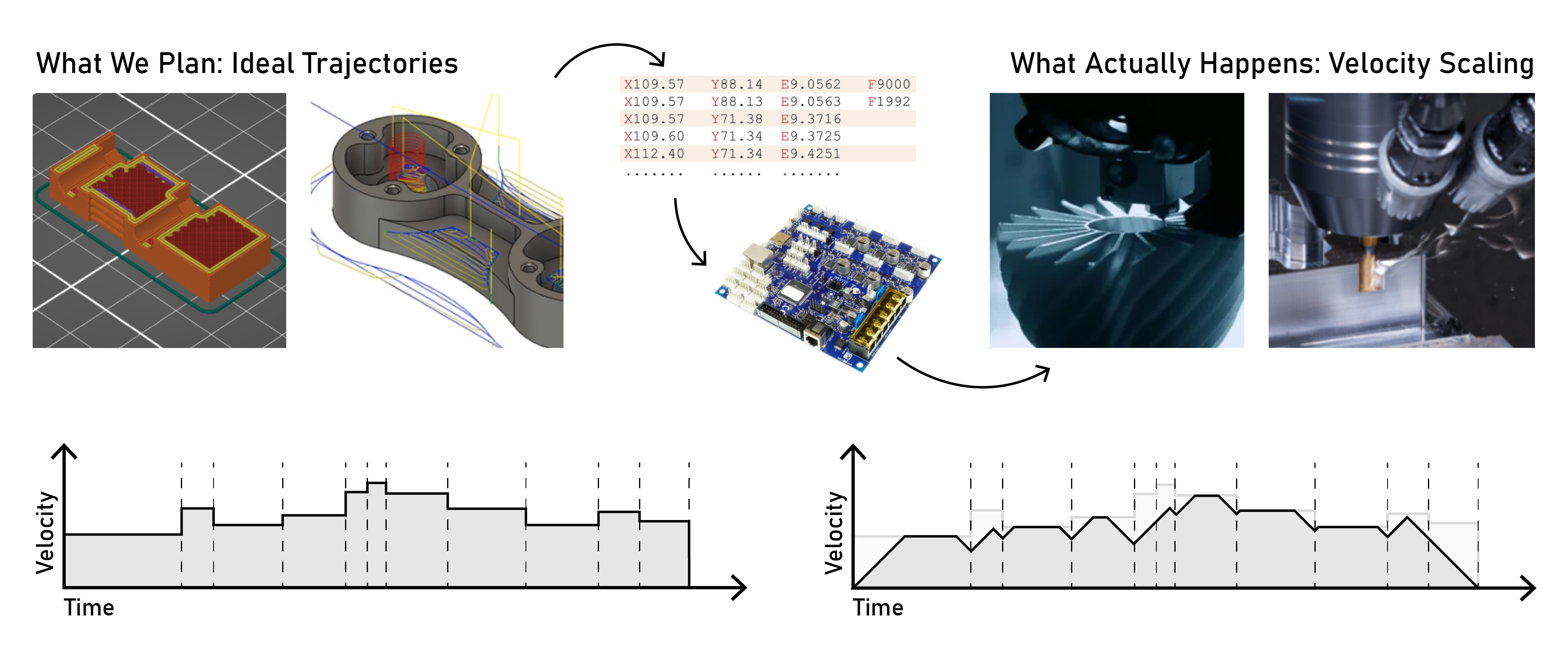
We know we want to minimize velocity deviations,
can we use models to design our machine accordingly?
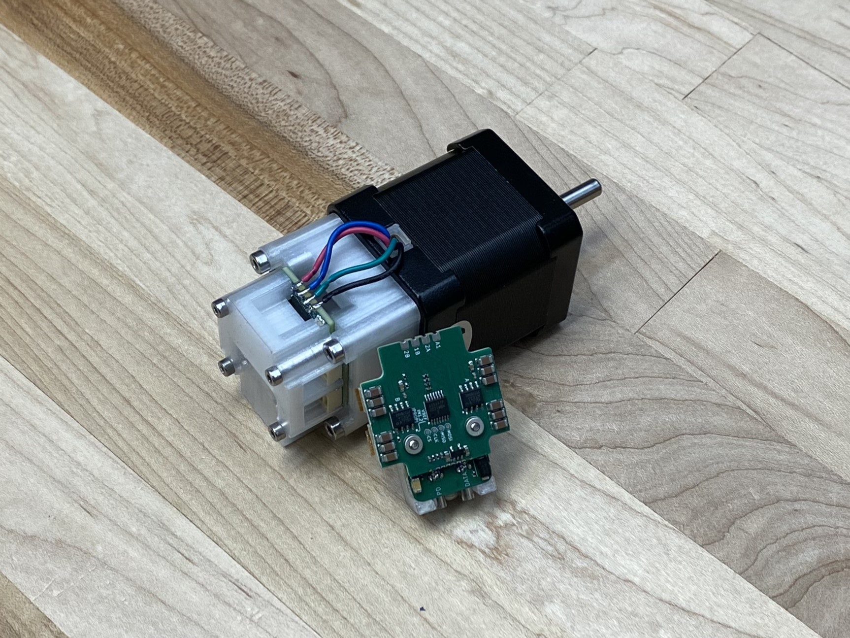
Closed-Loop Stepper Motor
Can we use just the motor to model itself?
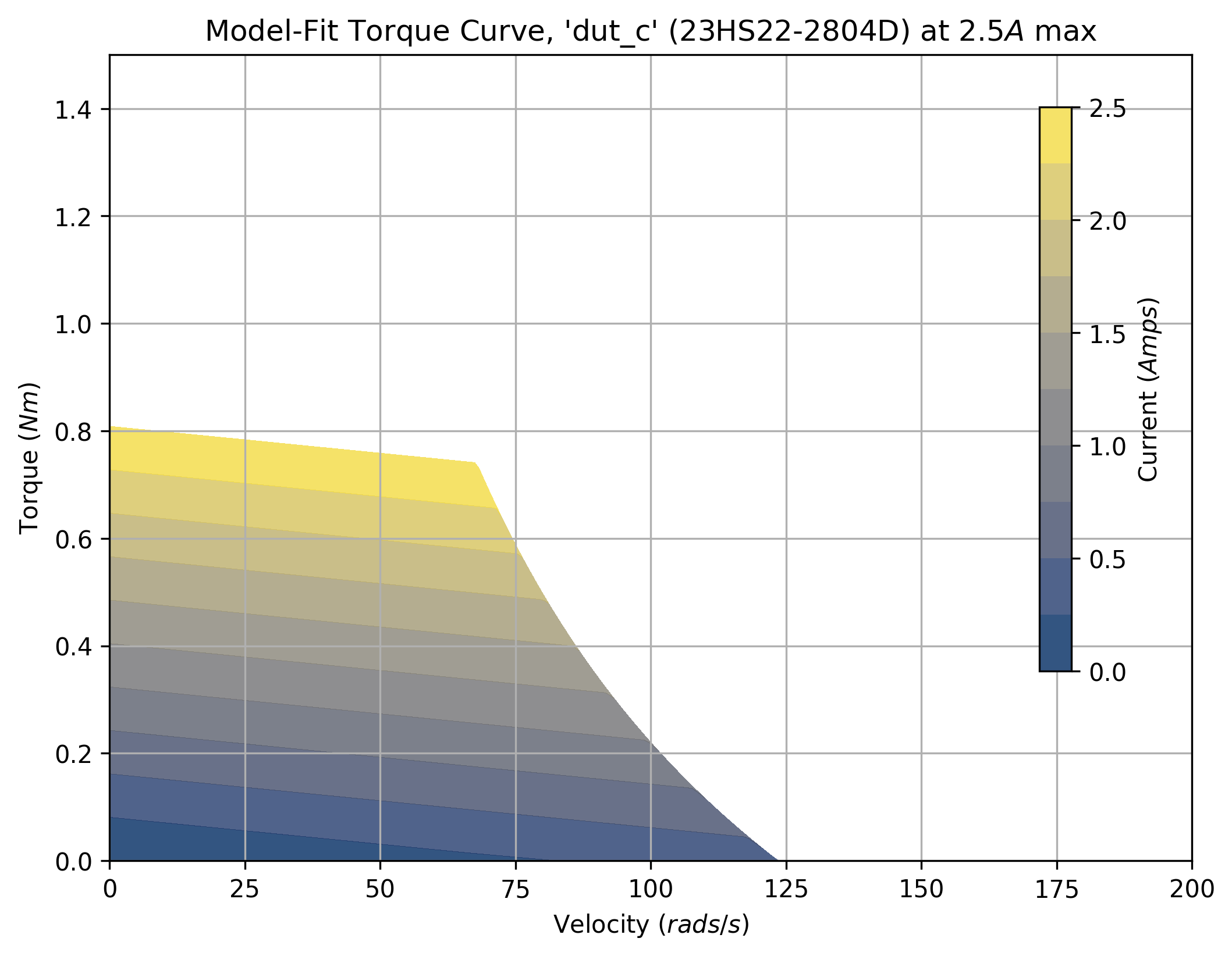
Motor Models
For any coil current, what torque does the motor produce?
For any motor speed and applied voltage, what current can we produce?
For any motor speed and applied voltage, what current can we produce?
Good models allow us to turn our machine's motors into sensors.
Mechanical Equations:
$$
\begin{aligned}
\tau &= k_tI \\
\dot{\omega}_m &= (\tau - k_d\omega_m) / J \\
\Theta &= \smallint \omega_m \, dt
\end{aligned}
$$
$\Theta (rads), \omega (rads/s), \dot{\omega} (rads/s^2)$ are pos, vel, and accel.
$\tau (Nm)$ is torque.
$J (kg \cdot m^2)$ is motor rotor inertia.
$\tau (Nm)$ is torque.
$J (kg \cdot m^2)$ is motor rotor inertia.
$k_t$ is the magic parameter; it allows us to estimate torque $(\tau, Nm)$
using our motor controller's current measurements $(I, Amps)$.
Electrical Equations:
$$
\begin{aligned}
Z &= \sqrt{R^2 + (\omega_e L)^2} \\
\omega_e &= \omega_m p \\
V_p &= V_a - k_e\omega_m \\
\dot{I} &= (V_p - RI) / L \\
I_{ss} &= V_a / Z
\end{aligned}
$$
$R (ohms), L (Henries)$ are motor resistance and inductance
$Z (ohms)$ is impedance, $V$ are voltages (applied, potential).
$Z (ohms)$ is impedance, $V$ are voltages (applied, potential).
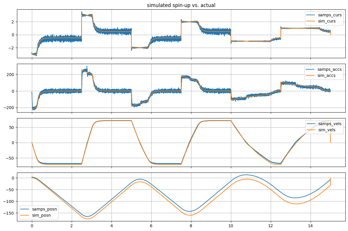
$k_t, k_e, k_d$ parameters are fit on time-series data from a spin-up test (above), using a known inertia
$R, L, J$ are measured by hand.
$R, L, J$ are measured by hand.
Kinematic Models: how machines move.
Kinematic Models: Mill
Mill Kinematics are simple: each motor moves one axis.
In general, we compute the inverse kinematics:
$$
\vec{X}_{actu} = f_{IK}(\vec{X}_{cart})
$$
These map end effector states $(\vec{X}_{actu})$
to actuator states $(\vec{X}_{cart})$
and include drive ratios: how motor rotations relate to linear translations.
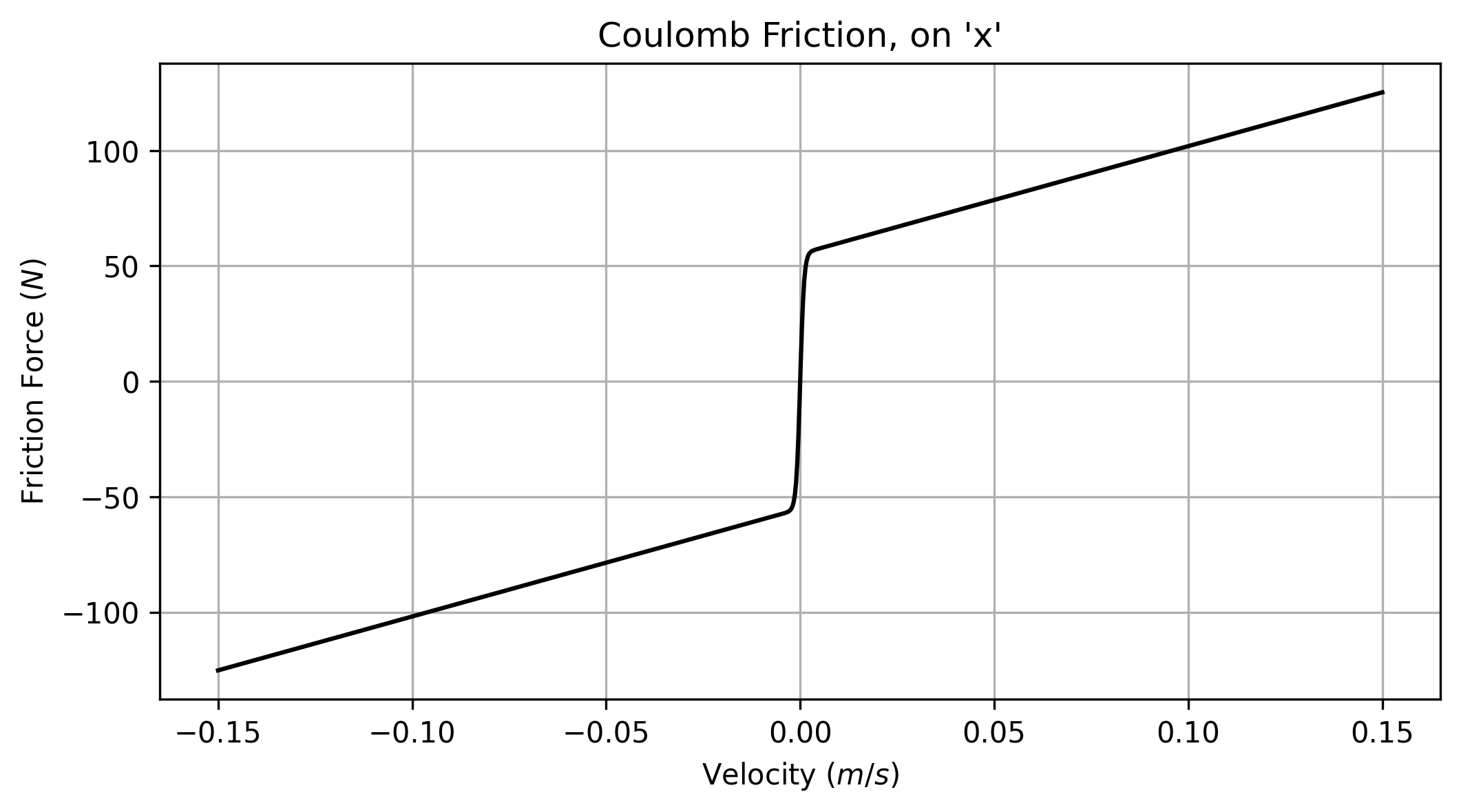
To model friction, I use a Coulomb approximation that includes stiction.
$$
Fc(\vec{V}, \mu_{visc}, \mu_{stick})
$$
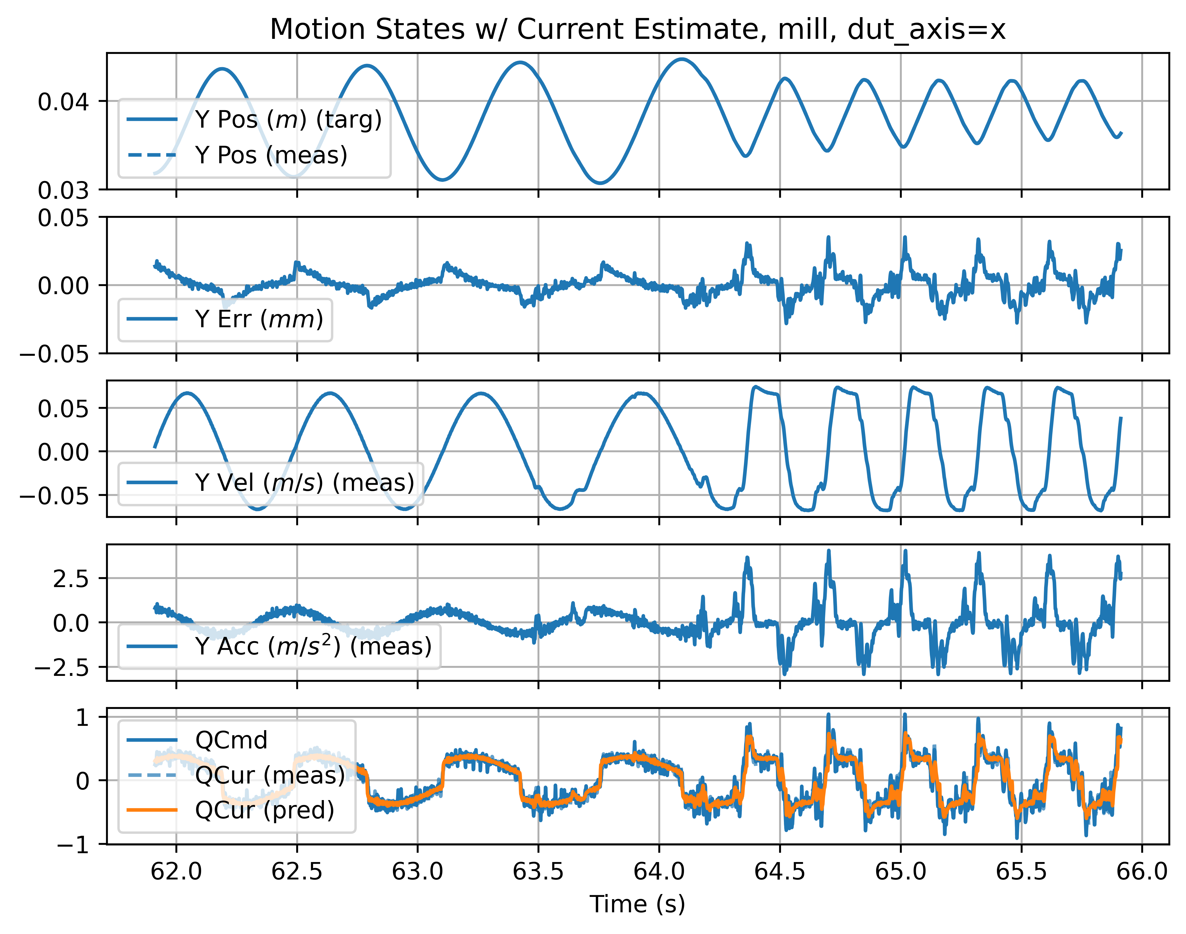
Parameters $(\mu_{visc}, \mu_{stick})$ are fit using time-series data (right).
The workup below translates from motion states
into actuator states and actuator currents:
$(\vec{V}_{cart}, \vec{A}_{cart}) \rightarrow (\vec{V}_{actu}, \vec{A}_{actu}, \vec{I}_{req,actu})$
$(\vec{V}_{cart}, \vec{A}_{cart}) \rightarrow (\vec{V}_{actu}, \vec{A}_{actu}, \vec{I}_{req,actu})$
$$
\begin{aligned}
\vec{F}_{req,cart} &= \vec{A}_{cart} \cdot m_{cart} + Fc(\vec{V}_{cart}) + 9.8 \cdot m_z \\
\vec{A}_{actu} &= f_{IK}(\vec{A}_{cart}) \\
\vec{\tau}_{rec,actu} &= f_{IK}(\vec{F}_{req,cart}) + \vec{A}_{actu} \cdot a_J \\
\vec{I}_{req,actu} &= \vec{\tau}_{rec,actu} / a_{kt} \\
\end{aligned}
$$
Kinematic Models: 3D Printer
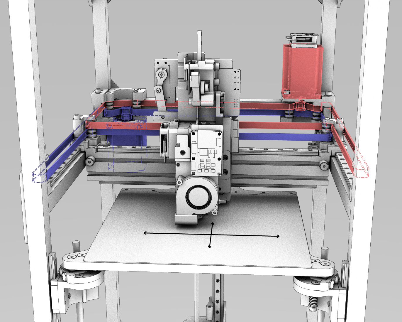
CoreXY Kinematics, which we will see in the 3D printing part of the thesis, mix axes and motors.
```python
# these defines transmission ratios,
rads_per_m = np.array([
    1.0 * (2.0 * np.pi) / 0.032, # a, b: 32mm per rot.
    1.0 * (2.0 * np.pi) / 0.032, # also: inverted,
    (2.0 * np.pi) / 0.008,       # z: 8mm per rotation
])

# this is the inverse kinematic (IK) implementation
def cart_2_actu_corexy(xyz):
    abz = np.array([
        (xyz[:, 0] - xyz[:, 1]) * rads_per_m[0],
        (xyz[:, 0] + xyz[:, 1]) * rads_per_m[1],
        (xyz[:, 2])             * rads_per_m[2],
    ])

    return abz
```
The controls framework that I develop allows us to describe and debug kinematics in high-level programming languages.
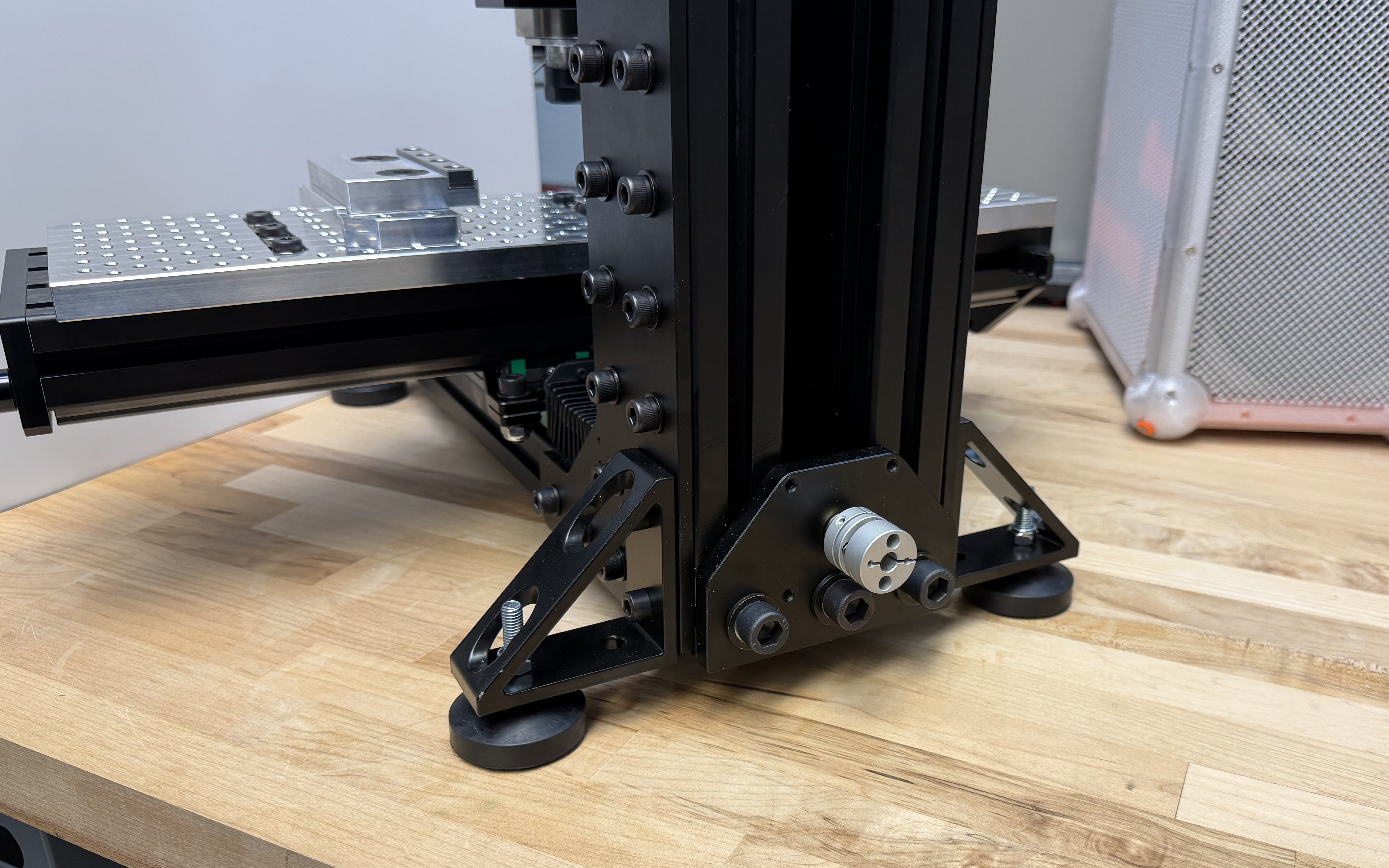
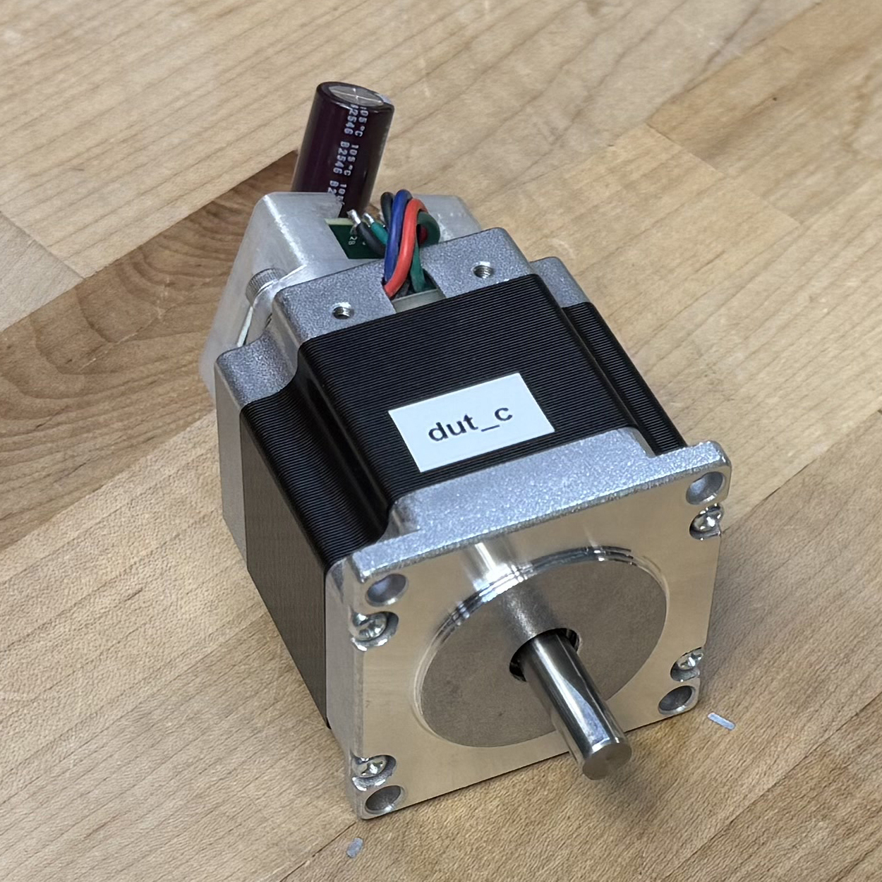
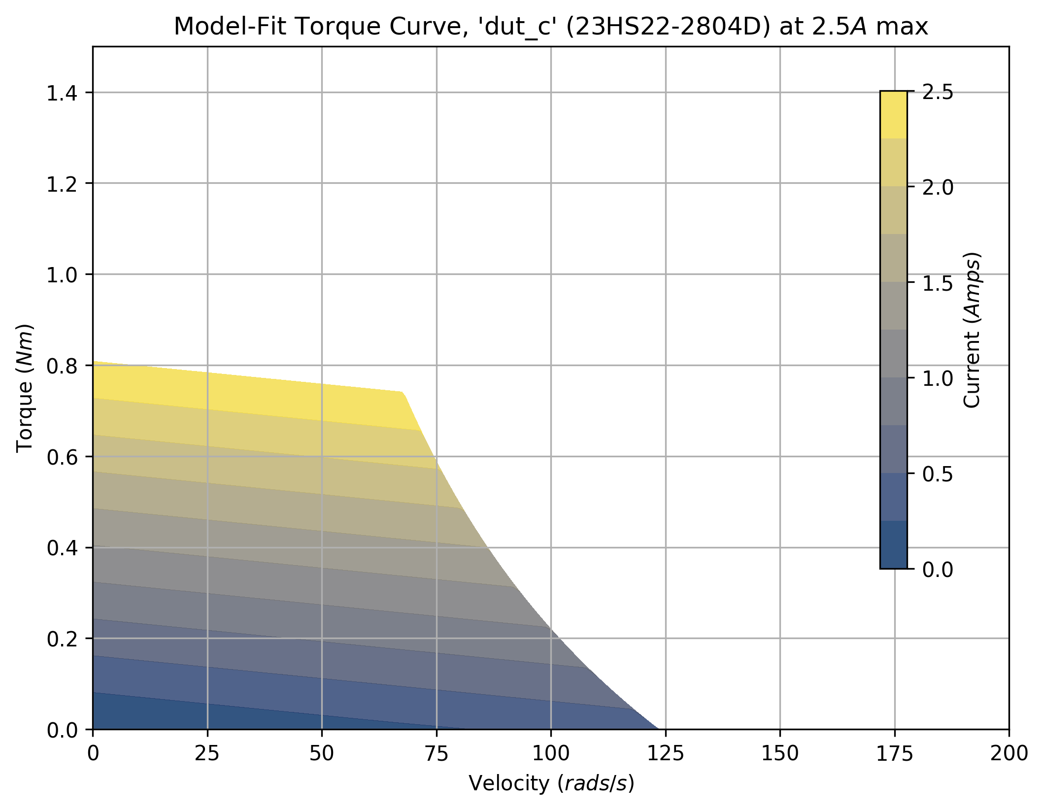
We can virtually combine axes and motors, to estimate the combinations' performance.
Force $=$ torque $\times$ drive ratio.
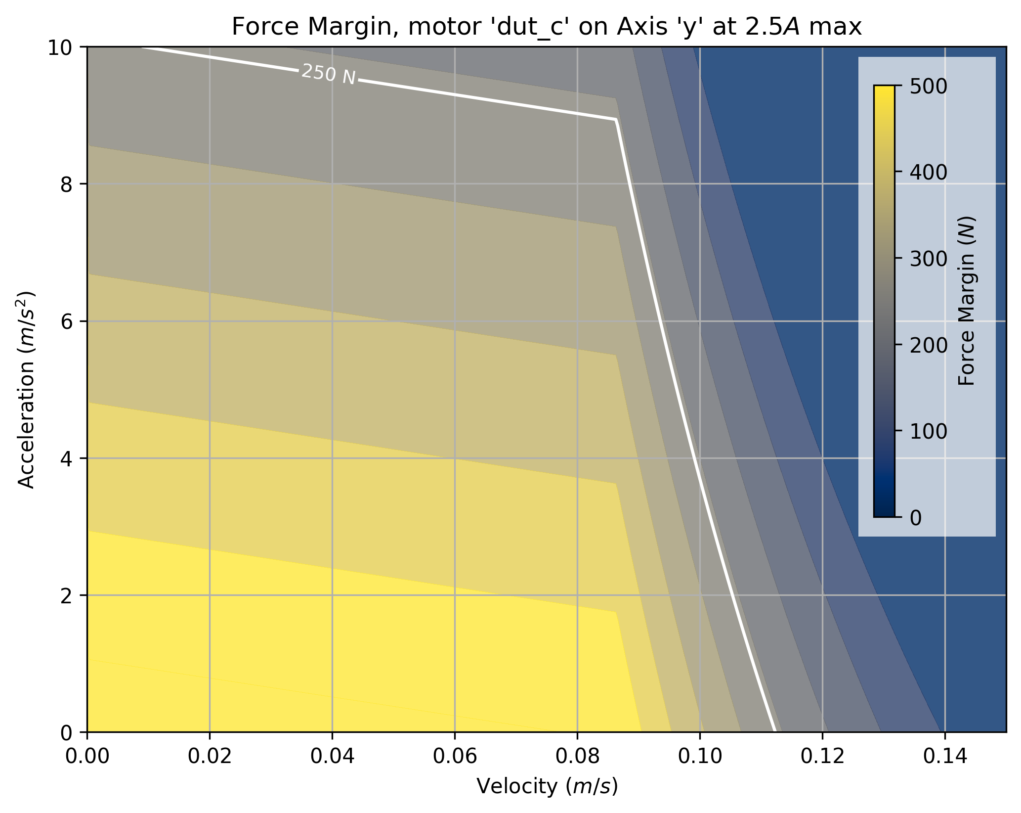
A force margin plot: for any velocity (x-axis) and acceleration (y-axis),
how much force will we have available for metal cutting?
Area below the marked contour will leave us with enough motor current
to provide $250N$ of cutting force.
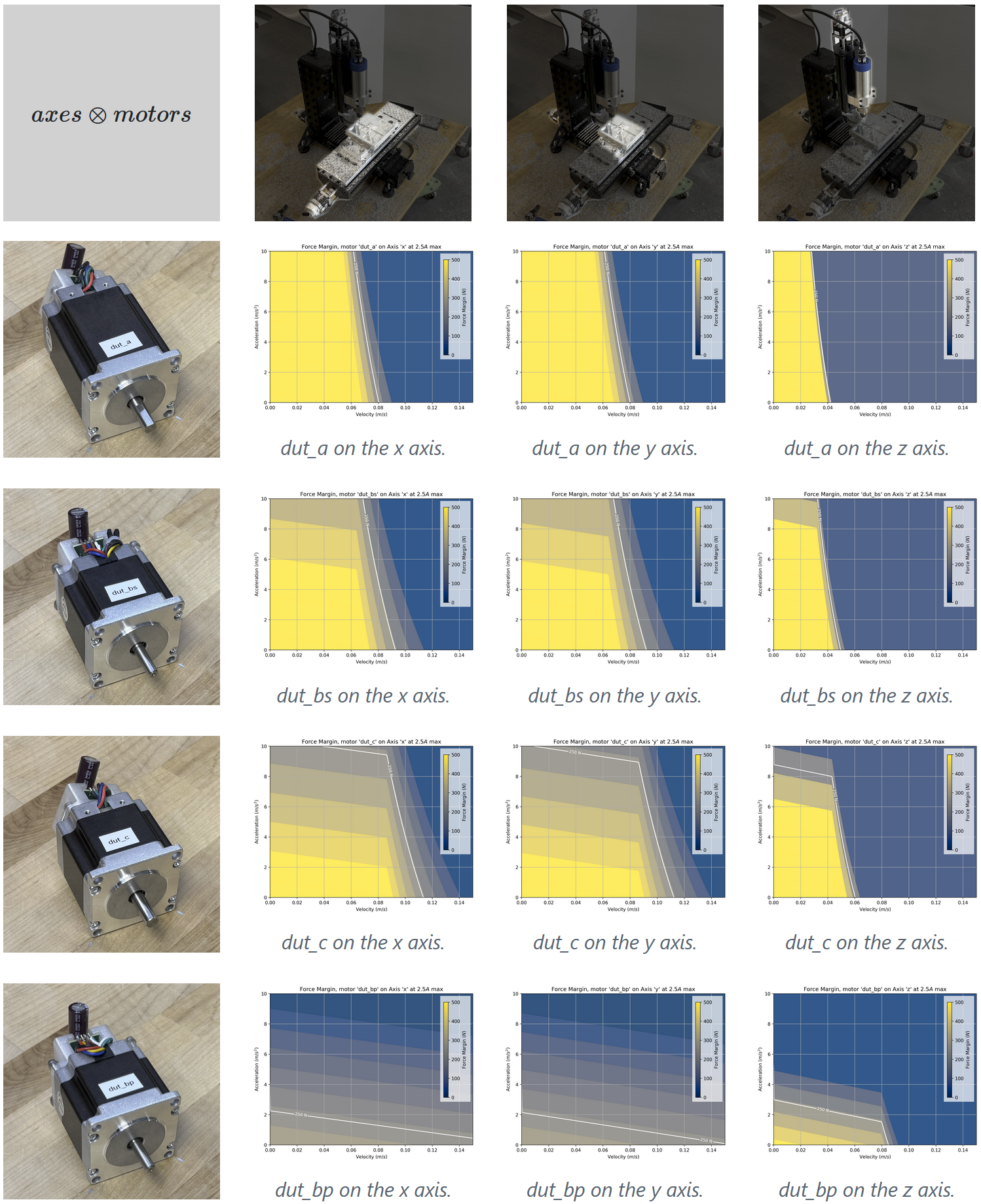
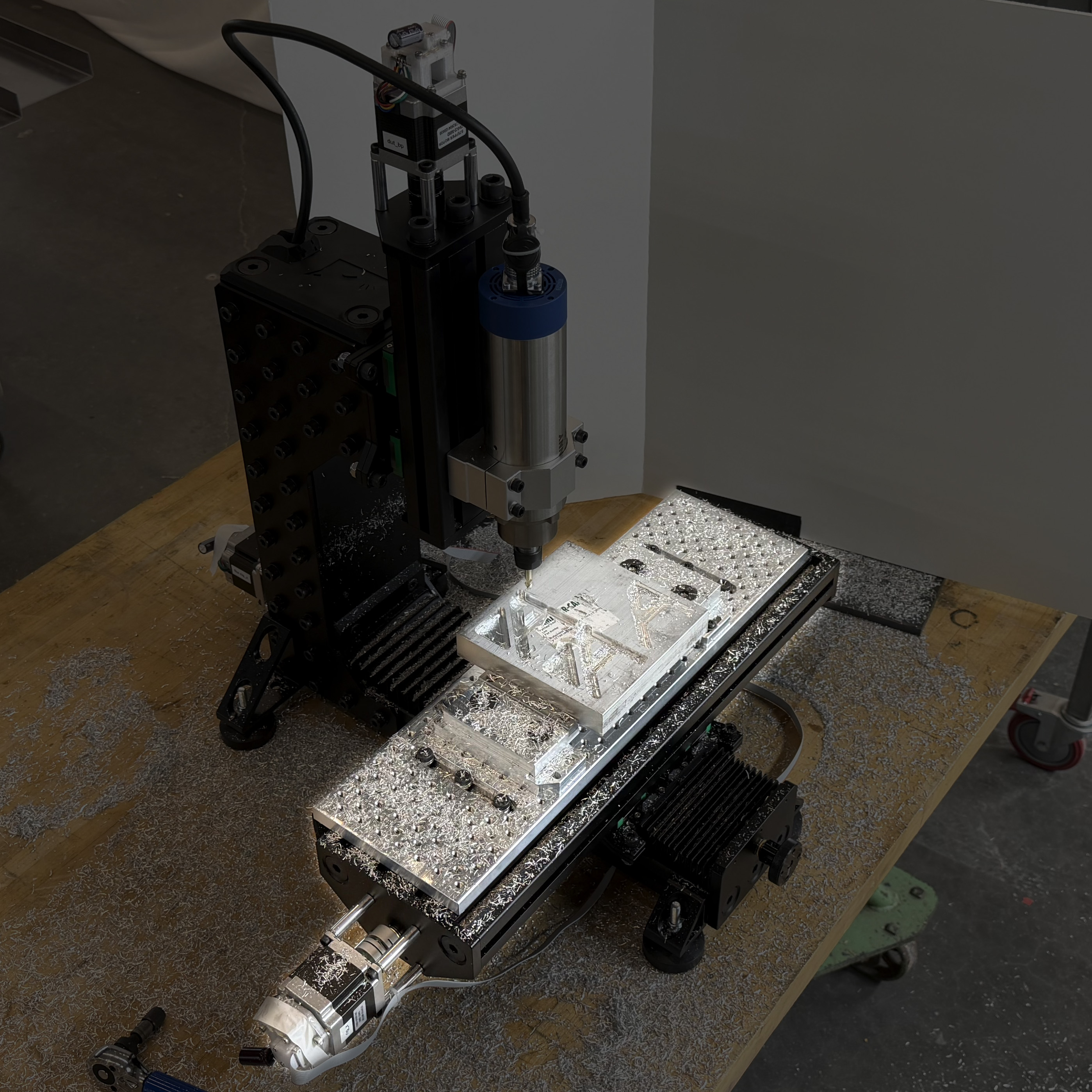
Models can help us to pick velocity controller parameters for $V_{max}, A_{max}$
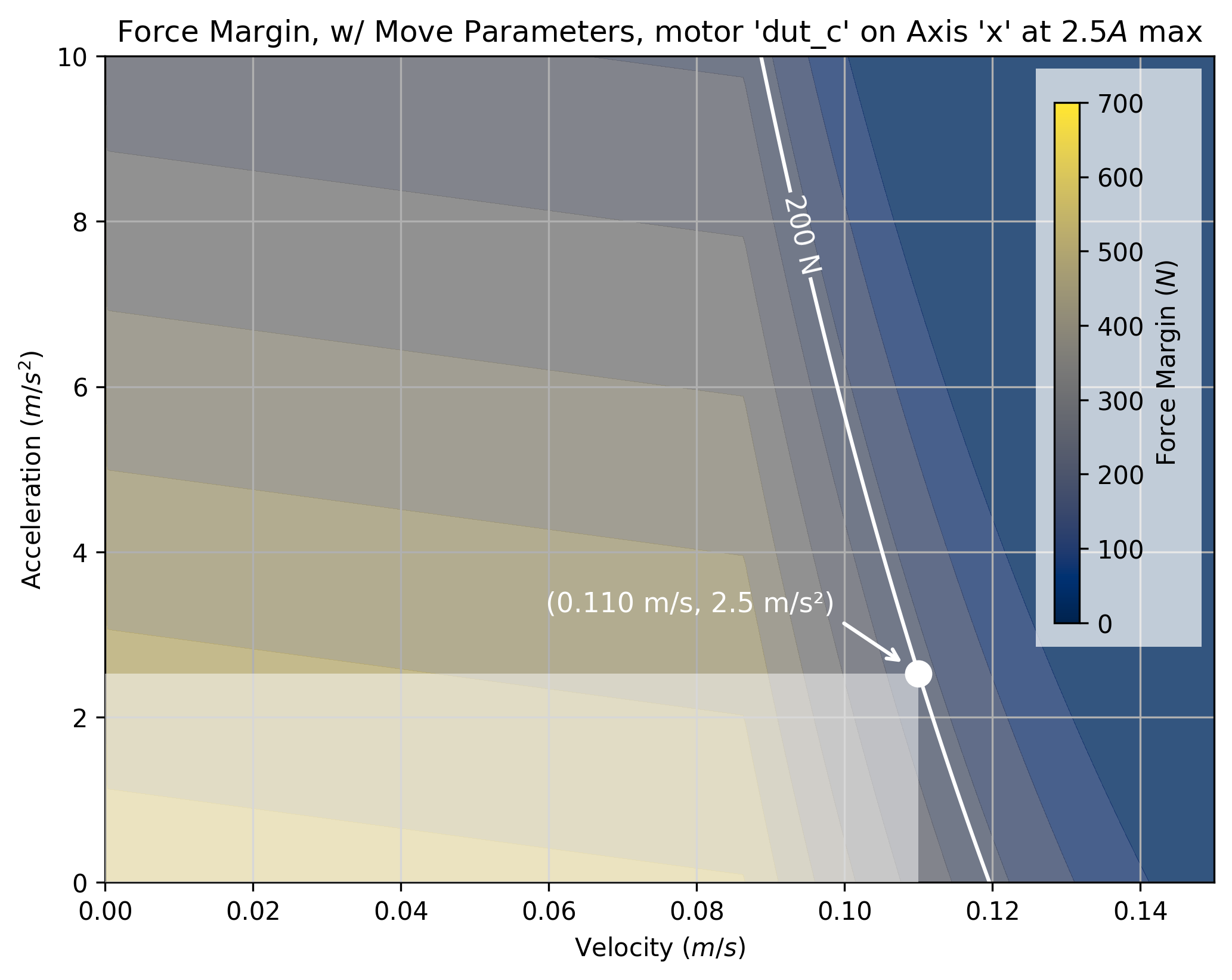
X-axis selection.
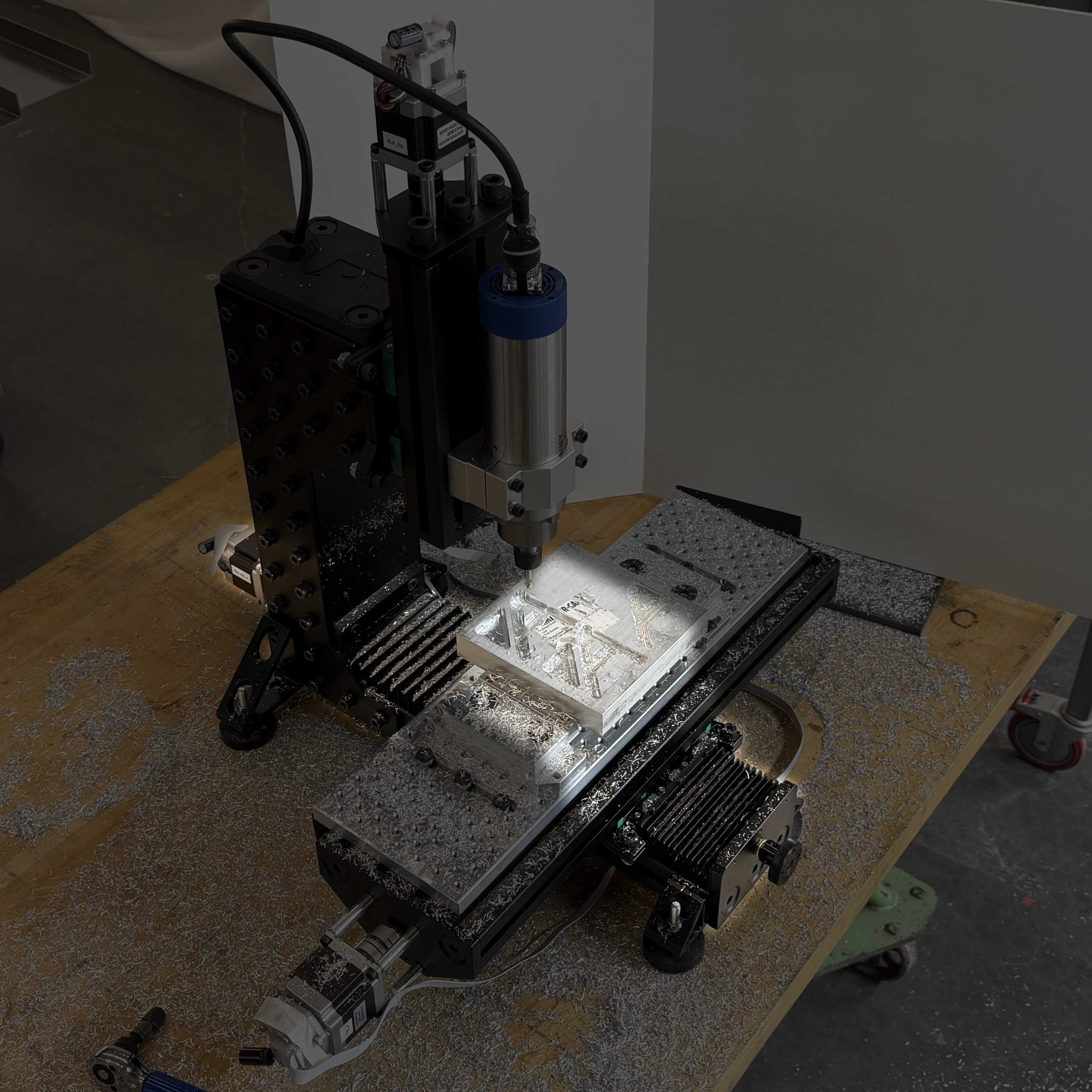
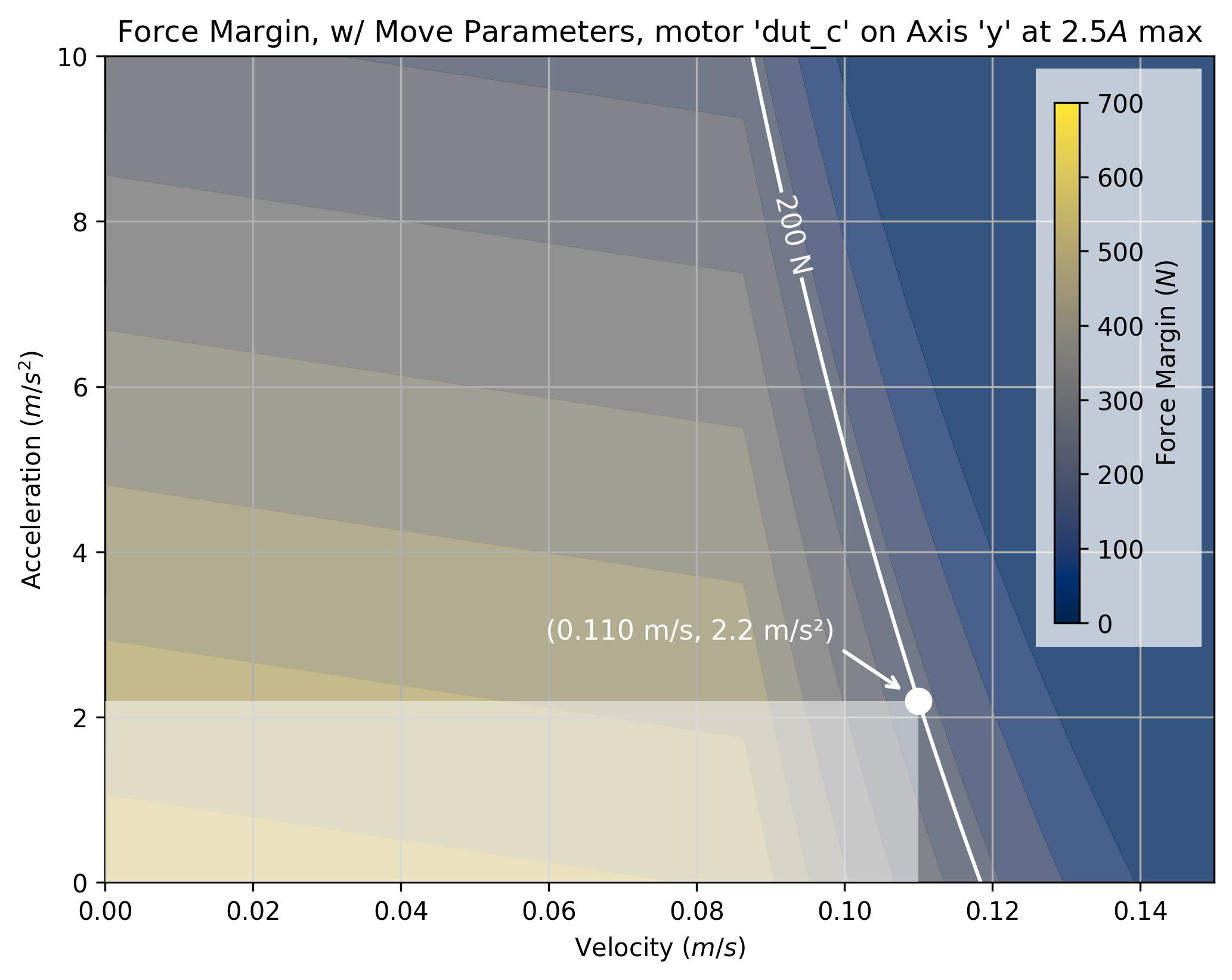
Y-axis selection.
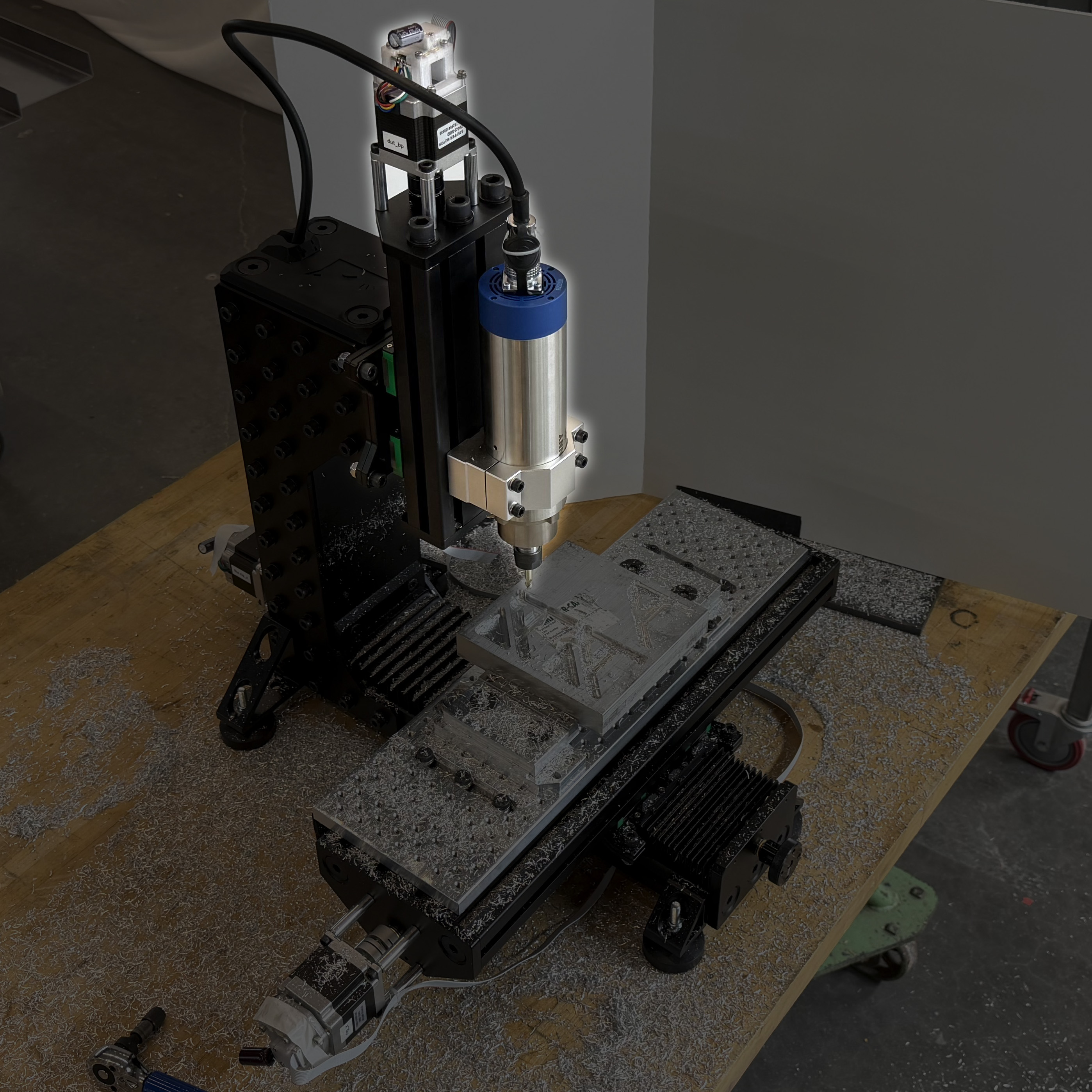
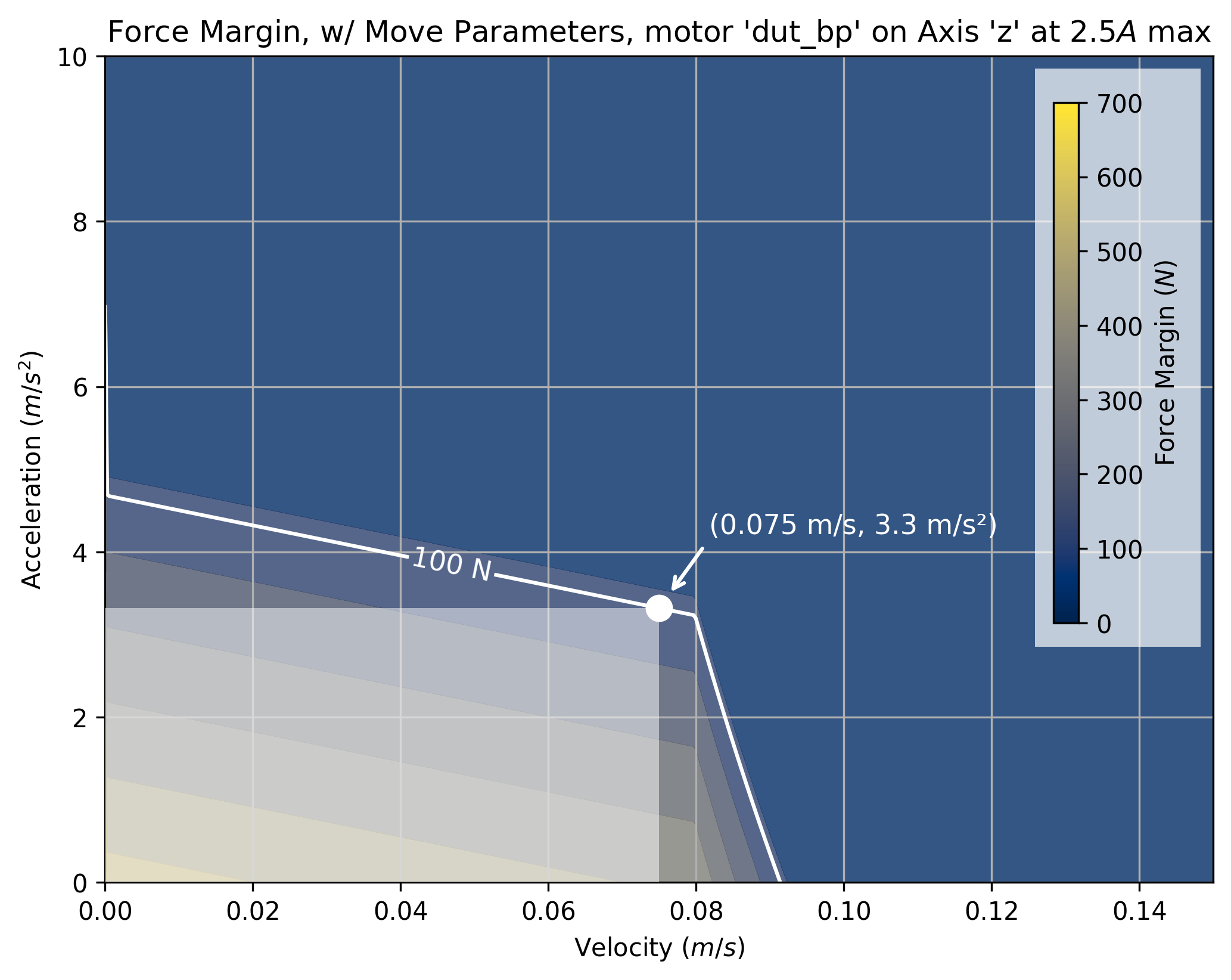
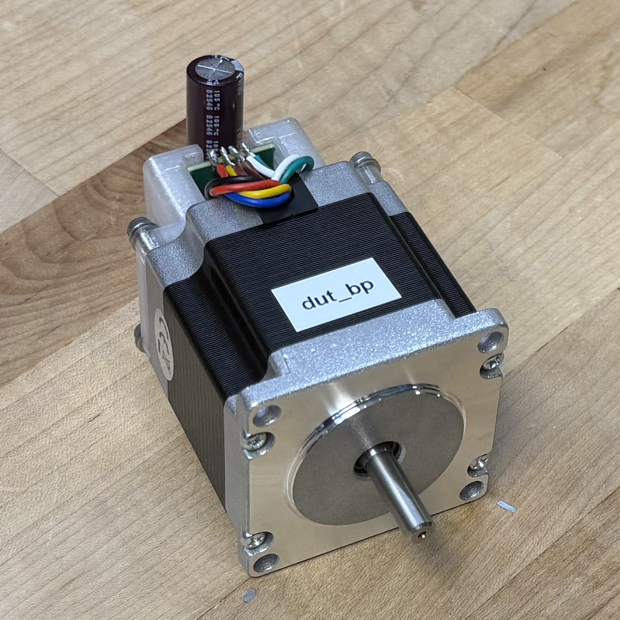
Z-axis selection.
| Axis | X | Y | Z |
| :--- | ---: | ---: | ---: |
| Force Margin $(N)$ | $200$ | $200$ | $100$ |
| Mfg. Motor Selection | LDO-57STH86 | LDO-57STH86 | LDO-57STH86 |
| Model-based Motor Selection | 23HS22-2804D | 23HS22-2804D | 23HS22-3008DP |
| | Mfg. $\rightarrow$ Mdl. | Mfg. $\rightarrow$ Mdl. | Mfg. $\rightarrow$ Mdl. |
| $V_{max}(mm/s)$ | $50 \rightarrow 110$ | $ 50 \rightarrow 110 $ | $ 25 \rightarrow 75 $ |
| $A_{max}(mm/s^2)$ | $300 \rightarrow 2500$ | $ 300 \rightarrow 2200 $ | $ 200 \rightarrow 3300 $ |
Table above: manufacturer $\rightarrow$ vs $\rightarrow$ model-based
for the machine's maximum velocities and accelerations $(V_{max}, A_{max}),$ per axis.
(big number good, small number bad).
(big number good, small number bad).
Model-based selections for $(V_{max}, A_{max})$ far exceed the kit manufacturer's recommendations.
| Name | X, Y (ours) | Z (ours) | Mfg. Spec (all) |
| :--- | ---: | ---: | ---: |
| Size | NEMA23x56 | NEMA23x56 | NEMA23x86 |
| $\tau_0$ | $1.20$ | $1.26$ | $2.45$ |
| $A_{max}$ | $2.80$ | $4.24$ | $3.00$ |
| $R (ohms)$ | $0.95$ | $0.38$ | $1.2$ |
| $L (mH)$ | $3.00$ | $1.10$ | $4.0$ |
| $J_{rot} (g \cdot cm^2)$ | $300$ | $300$ | $670$ |
| $k_t$ | $0.323$ | $0.193$ | n/a |
| $k_e$ | $0.331$ | $0.245$ | n/a |
| $k_d$ | $0.00093$ | $0.0010$ | n/a |
| $v_{max} (rads/s)$ | $125$ | $165$ | n/a |
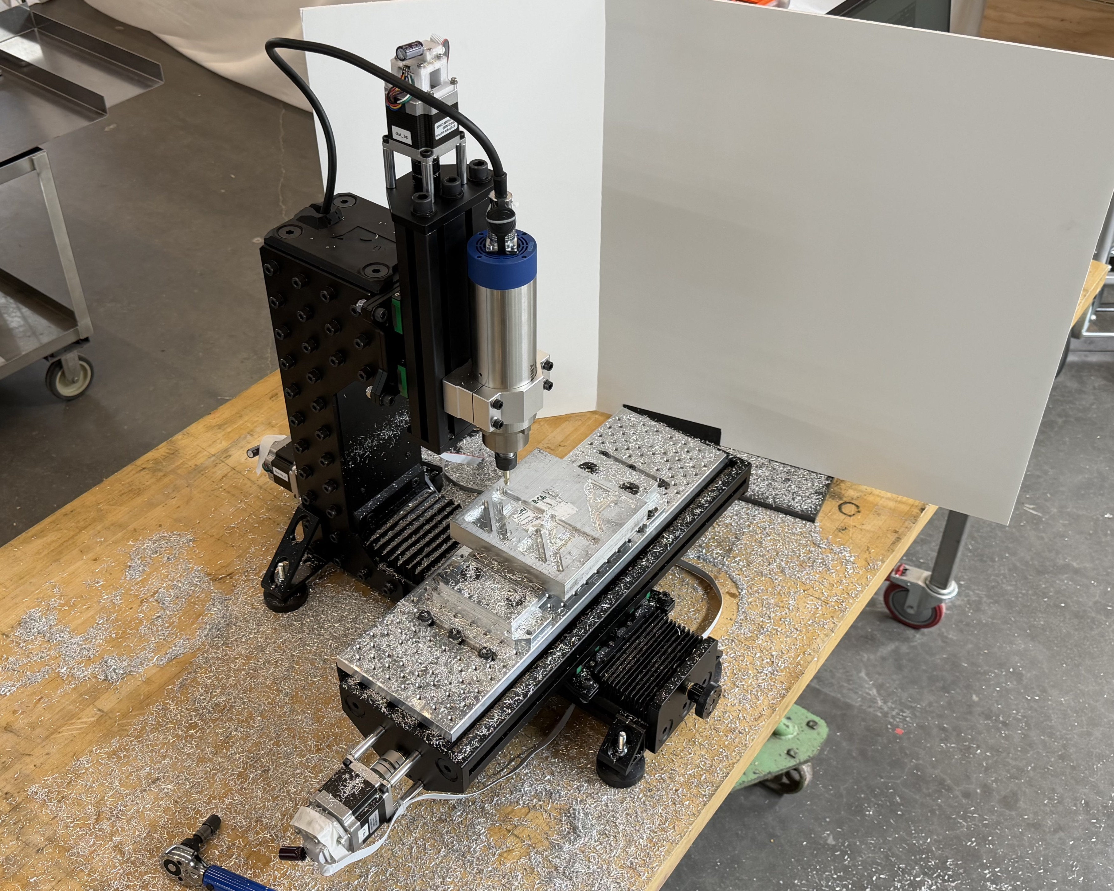
Machining the pocket toolpath, trapezoidal motion solver.
Machining the adaptive toolpath. As the machine is running, we collect data from the motor controllers...
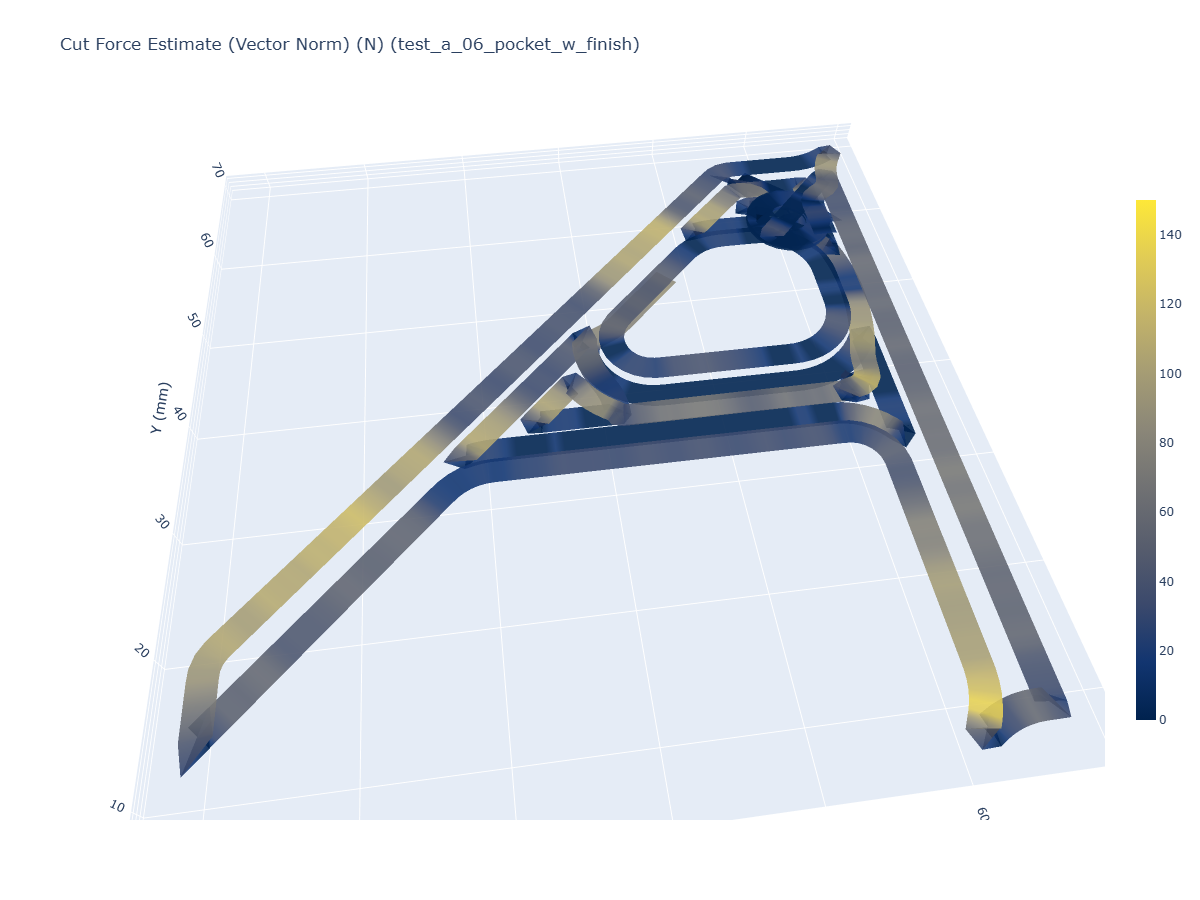
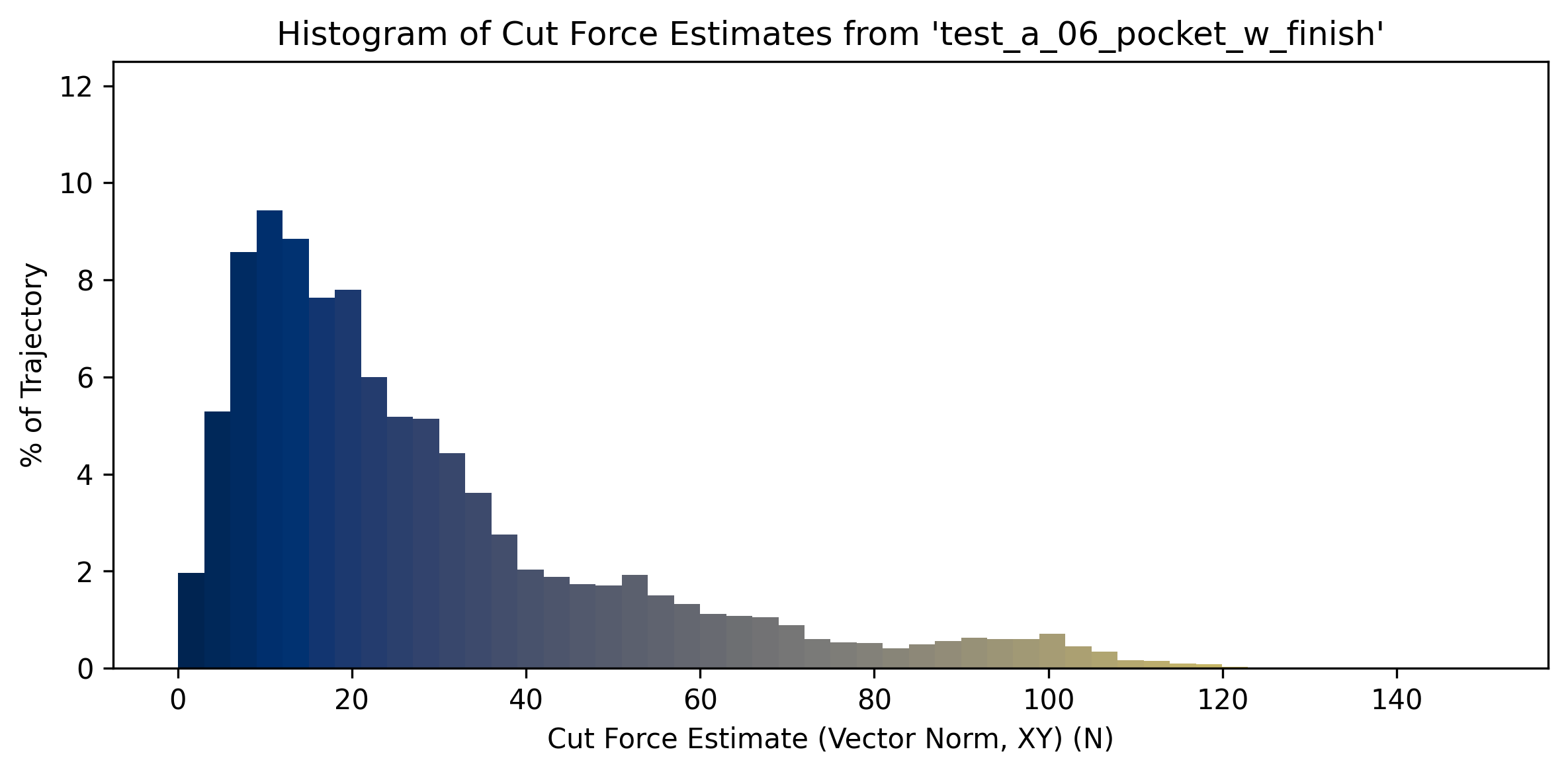
We can use that data to make cut force estimates, *
These are generated from the pocket toolpath.
These are generated from the pocket toolpath.
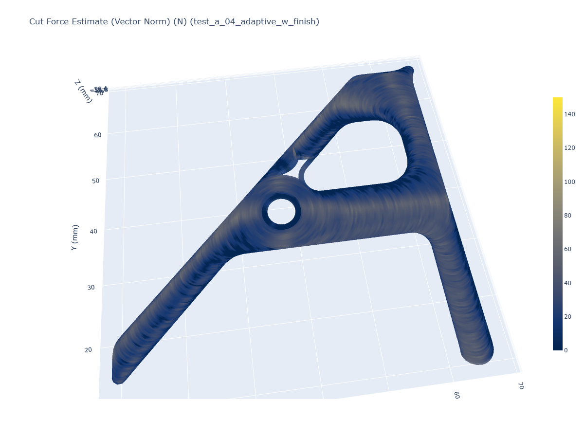
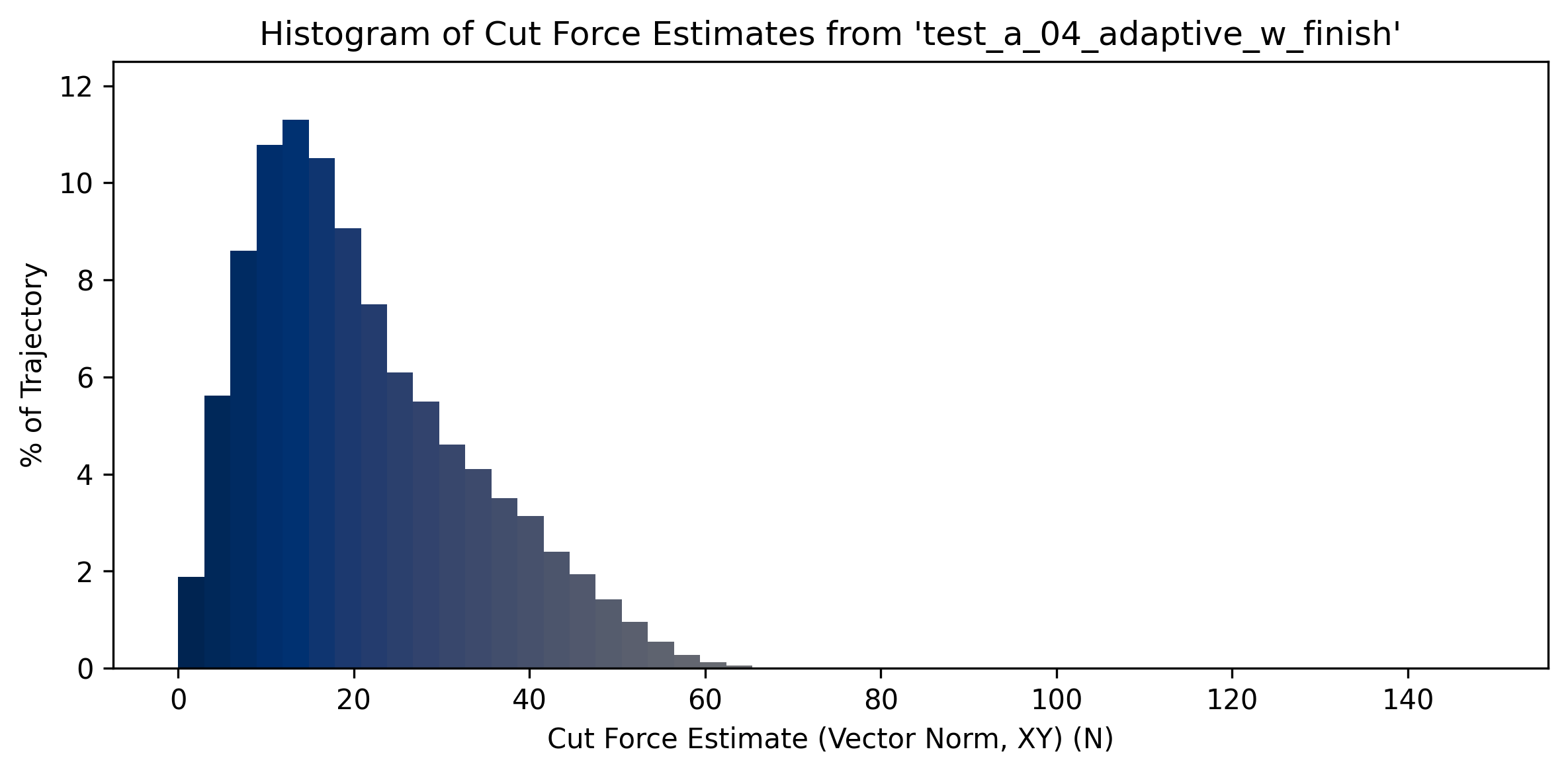
Cut force estimates, adaptive toolpath.
Models can be used in the machine design process, helping us to
make choices with data based on our particular hardware.
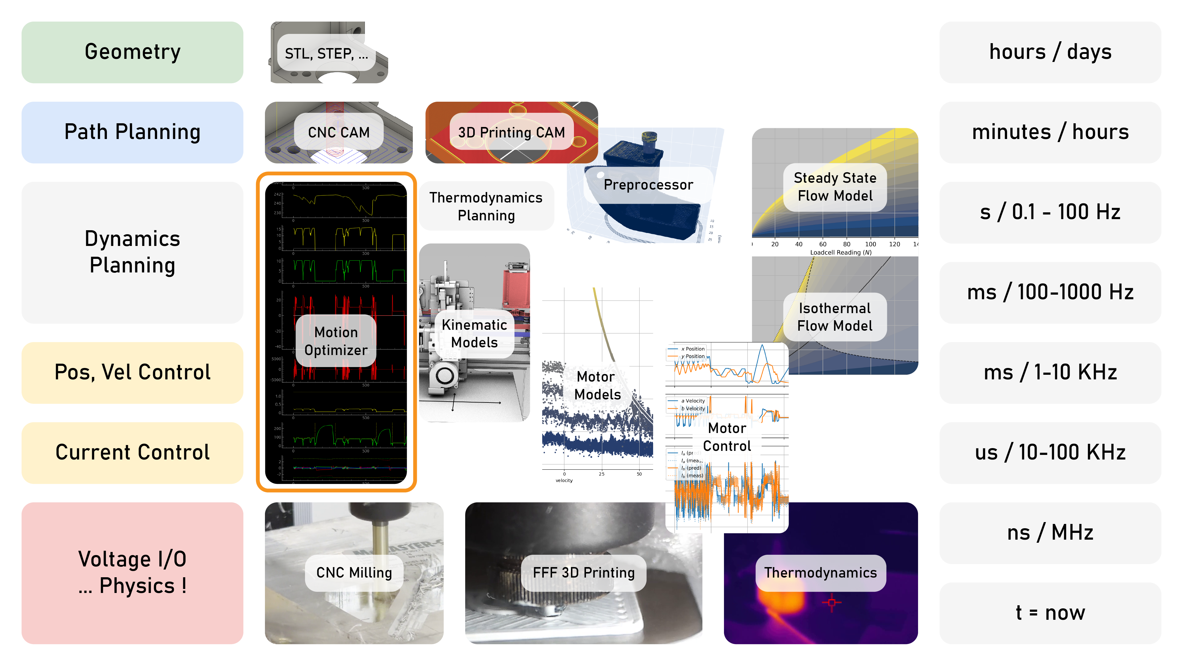
Software-defined controllers let us inspect toolpaths before we run them.
Motion and kinematic models, when combined with time-series data from motors and
motion controllers, can be combined to produce new measurements, like cut force.
Can we use models directly, to improve our machine's performance?
Here is force margin for our mill's $x$ axis.
These plots only show positive accelerations (speeding up).
These plots only show positive accelerations (speeding up).
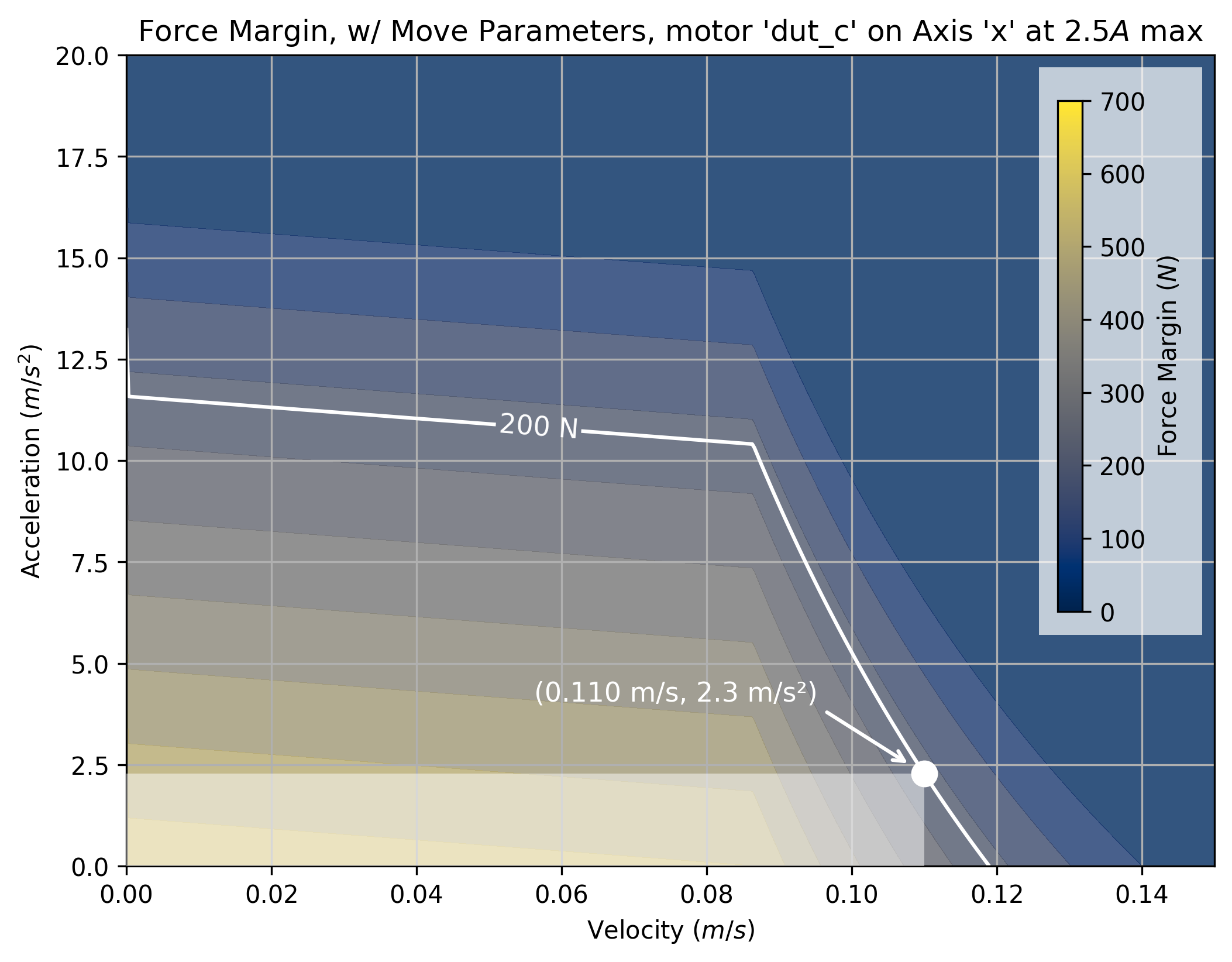
Force margin for our mill's $x$ axis.
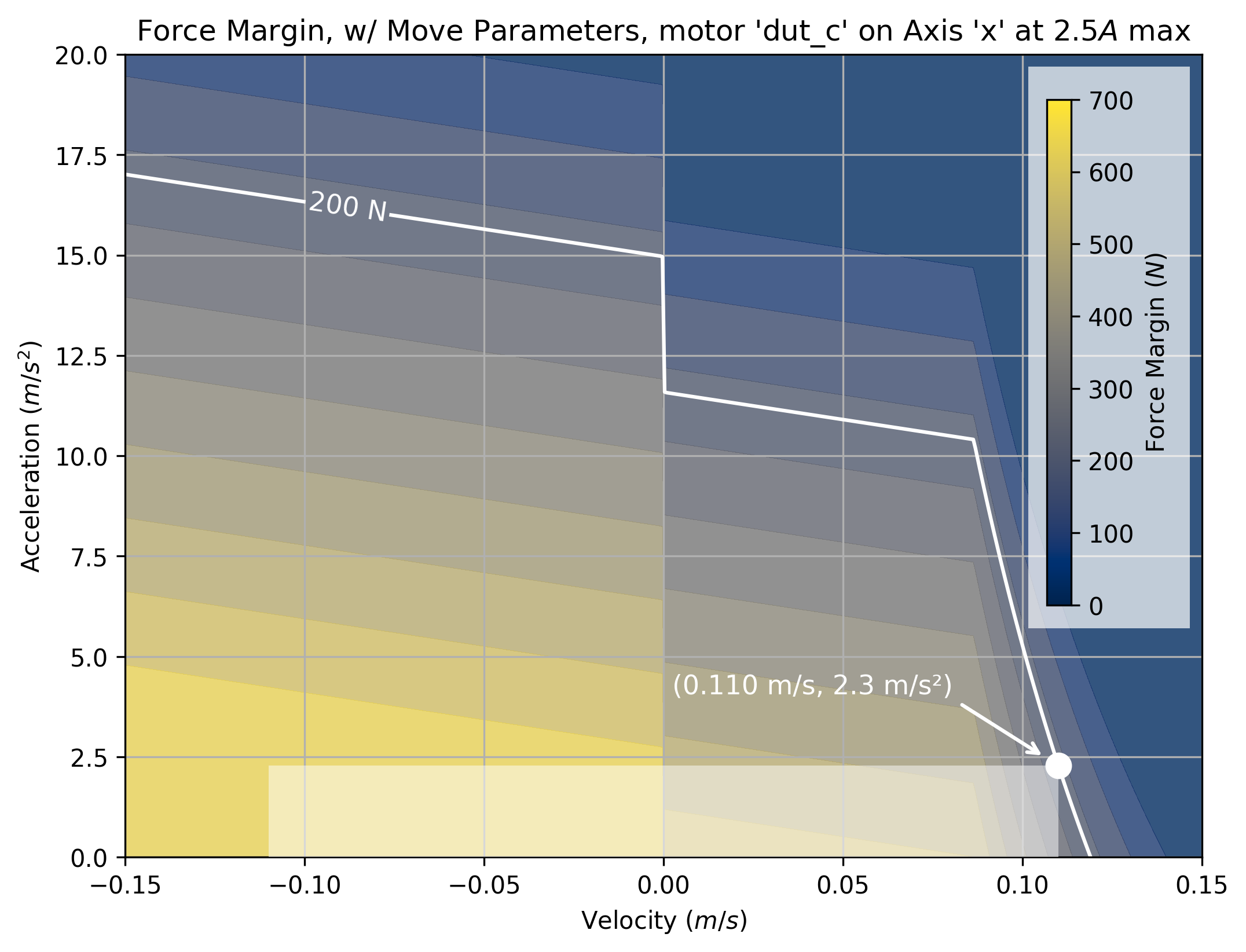
Here we see negative accelerations (i.e. braking, left half of plot) as well.
Here we see negative accelerations (i.e. braking, left half of plot) as well.
Model-based velocity solver. 2D Trajectory at left, solution states at right, top to bottom:
solver gradients, $v(s)$, $\Delta t(s)$, $I_{req}(s)$, $\dot{I}_{req}(s)$, $\vec{V}(t)$, and convergence.
solver gradients, $v(s)$, $\Delta t(s)$, $I_{req}(s)$, $\dot{I}_{req}(s)$, $\vec{V}(t)$, and convergence.
We provide...
$$
\overset{\vec{x}(s)}{\begin{bmatrix} 0 \\ \vdots \\ \vdots \\ \vdots \\ n \end{bmatrix}}
\
\overset{v_{max}(s)}{\begin{bmatrix} 0 \\ \vdots \\ \vdots \\ \vdots \\ n \end{bmatrix}}
\
\overset{I_{prop}(s)}{\begin{bmatrix} 0 \\ \vdots \\ \vdots \\ \vdots \\ n \end{bmatrix}}
\
\overset{\dot{I}_{prop}(s)}{\begin{bmatrix} 0 \\ \vdots \\ \vdots \\ \vdots \\ n \end{bmatrix}}
$$
Target trajectory, encoded in equal-size steps $\Delta d$ through space $s$
$\vec{x}$ positions
$v_{max}$ rate limits
$I_{prop}$ current deployment scalars
$\dot{I}_{prop}$ current slewrate scalars
$\vec{x}$ positions
$v_{max}$ rate limits
$I_{prop}$ current deployment scalars
$\dot{I}_{prop}$ current slewrate scalars
Solver selects:
$$
\overset{v(s)}{\begin{bmatrix} 0 \\ \vdots \\ \vdots \\ \vdots \\ n \end{bmatrix}}
$$
Velocities at each point, $v(s)$
We calculate ...
$$
\begin{aligned}
\vec{v}_i &= v_{(s)} \cdot \hat{v}_{(s)} \\
\vec{v}_f &= v_{(s + 1)} \cdot \hat{v}_{(s+1)} \\
v_f &= \text{proj}_{\vec{v}_f}\hat{v}_i \\
\Delta t &= \Delta d / (\frac{1}{2} (v_f + v_i)) \\
\Delta t &= \text{softclamp}(\Delta t, t_{min}, t_{max}) \\
\vec{a}_{req} &= (\vec{v}_f - \vec{v}_i) / \Delta t \\
\end{aligned}
$$
The required acceleration $\vec{a}_{req}$
to accomplish solver's choice of $v(s)$ along the trajectory $\vec{x}(s)$
And ...
$$
\overset{I_{req}(s)}{\begin{bmatrix} 0 \\ \vdots \\ \vdots \\ \vdots \\ n \end{bmatrix}}
\
\overset{I_{lim}(s)}{\begin{bmatrix} 0 \\ \vdots \\ \vdots \\ \vdots \\ n \end{bmatrix}}
\
\overset{\dot{I}_{req}(s)}{\begin{bmatrix} 0 \\ \vdots \\ \vdots \\ \vdots \\ n \end{bmatrix}}
\
\overset{\dot{I}_{lim}(s)}{\begin{bmatrix} 0 \\ \vdots \\ \vdots \\ \vdots \\ n \end{bmatrix}}
$$
The required and available actuator currents, and current slew rates.
This step uses kinematic models and actuator models.
Real limits are scaled by $I_{prop}, \dot{I}_{prop}$, heuristics!
Real limits are scaled by $I_{prop}, \dot{I}_{prop}$, heuristics!
Finally !
$$
\begin{aligned}
\text{cost}&=\sum_{s} \Bigl[\, I_{2big}(s) \Bigr] + \sum_{s} \Bigl[\, \Delta t(s) \Bigr] \\
\end{aligned} \\
\min_{v(s)} \; \text{cost}
$$
Sum all actuator constaints exceeded $(I_{2big})$, and total time; all $\Delta t(s)$.
Minimize the cost function by optimizing over $v(s)$.
The solver can use more of our machines's dynamic range.
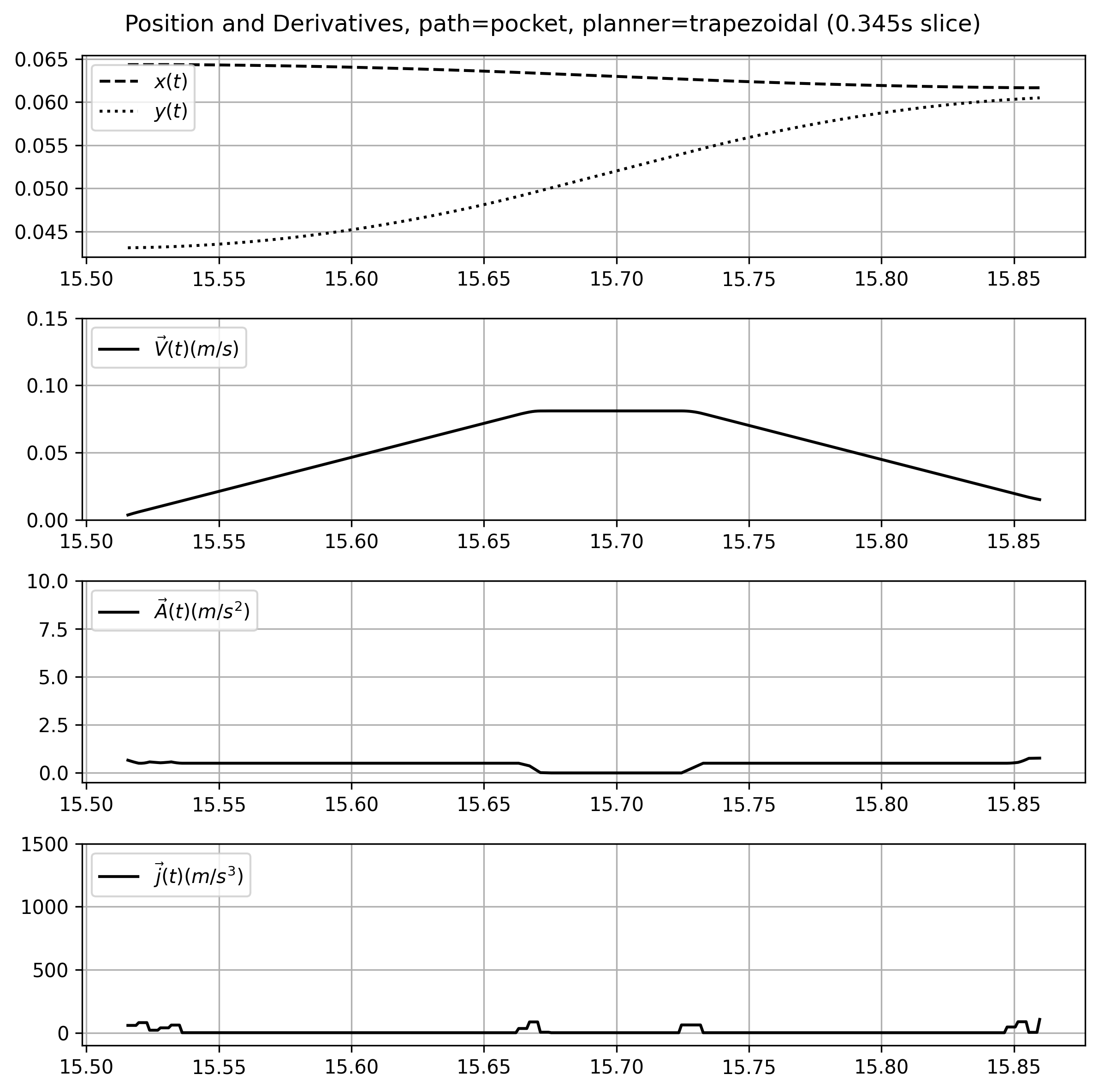
Motion states: position, velocity, acceleration, and jerk.
One segment from the trapezoid solver.
One segment from the trapezoid solver.
Motion states: position, velocity, acceleration, and jerk.
One segment from the model-based solver.
One segment from the model-based solver.
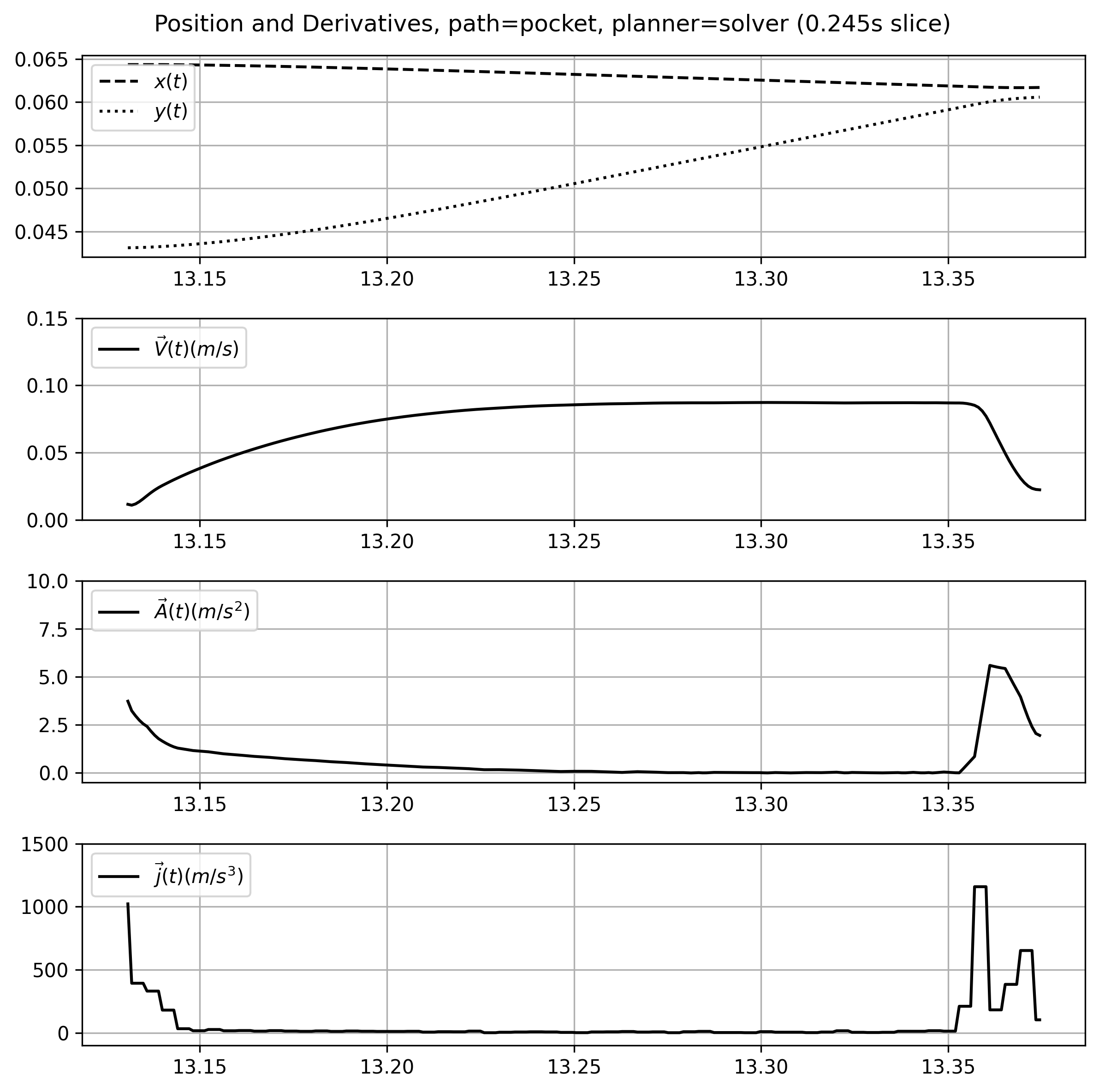
Same segment in less time, variable acceleration, more brakes than gas.
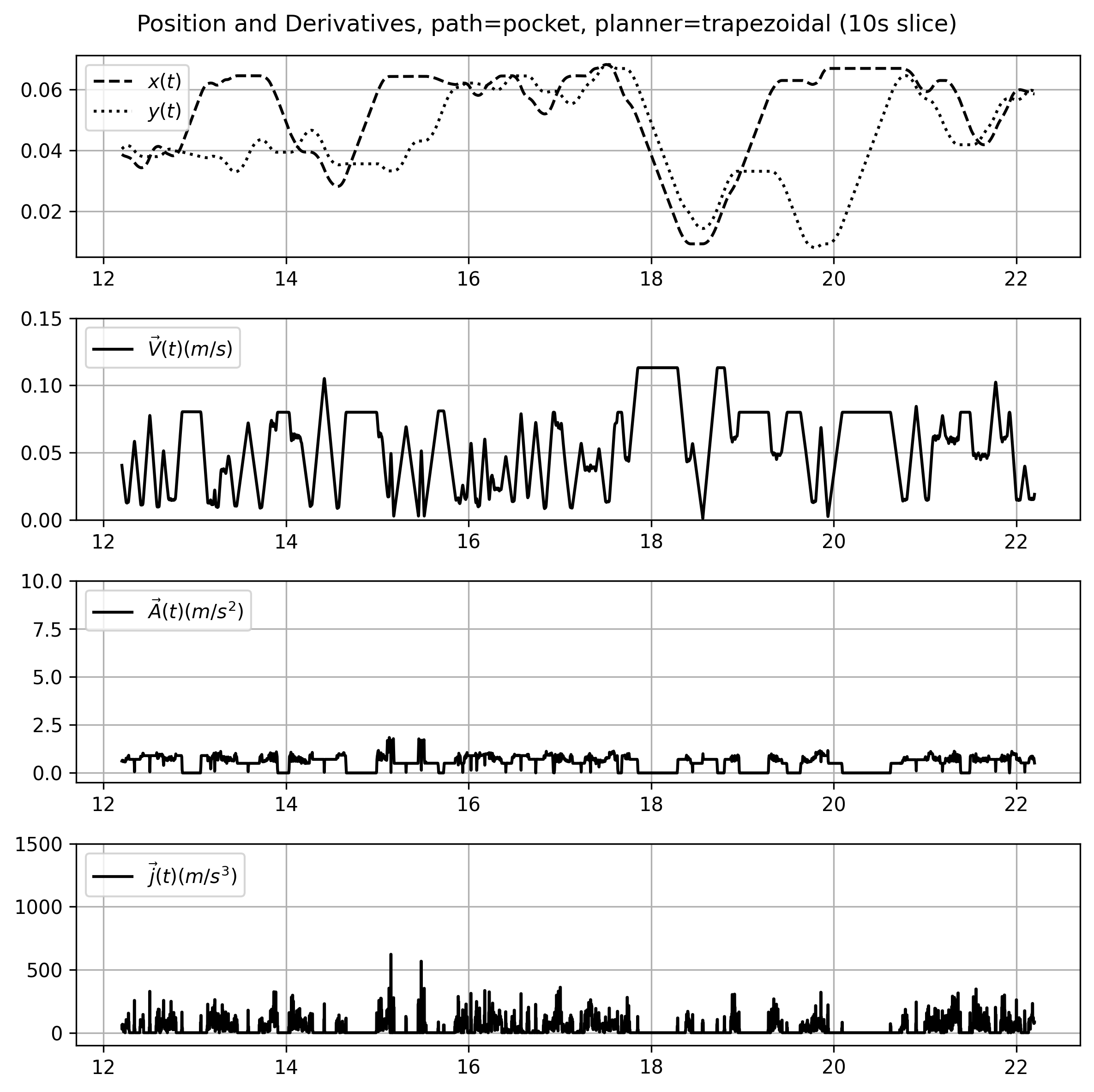
Motion states: position, velocity, acceleration, and jerk.
Multiple segments from the trapezoid solver.
Multiple segments from the trapezoid solver.
Motion states: position, velocity, acceleration, and jerk.
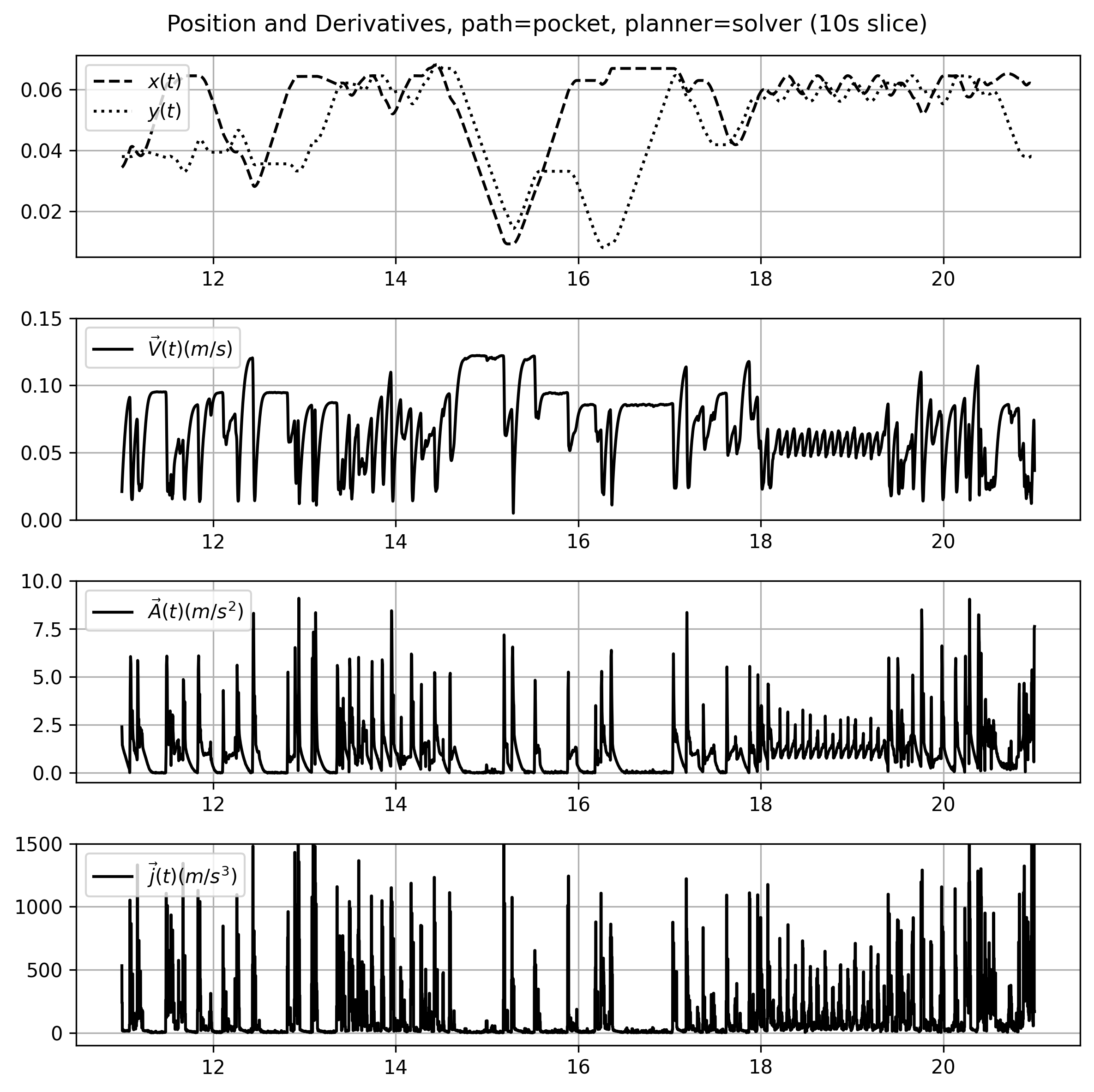
Multiple segments from the model-based solver.
Multiple segments from the model-based solver.
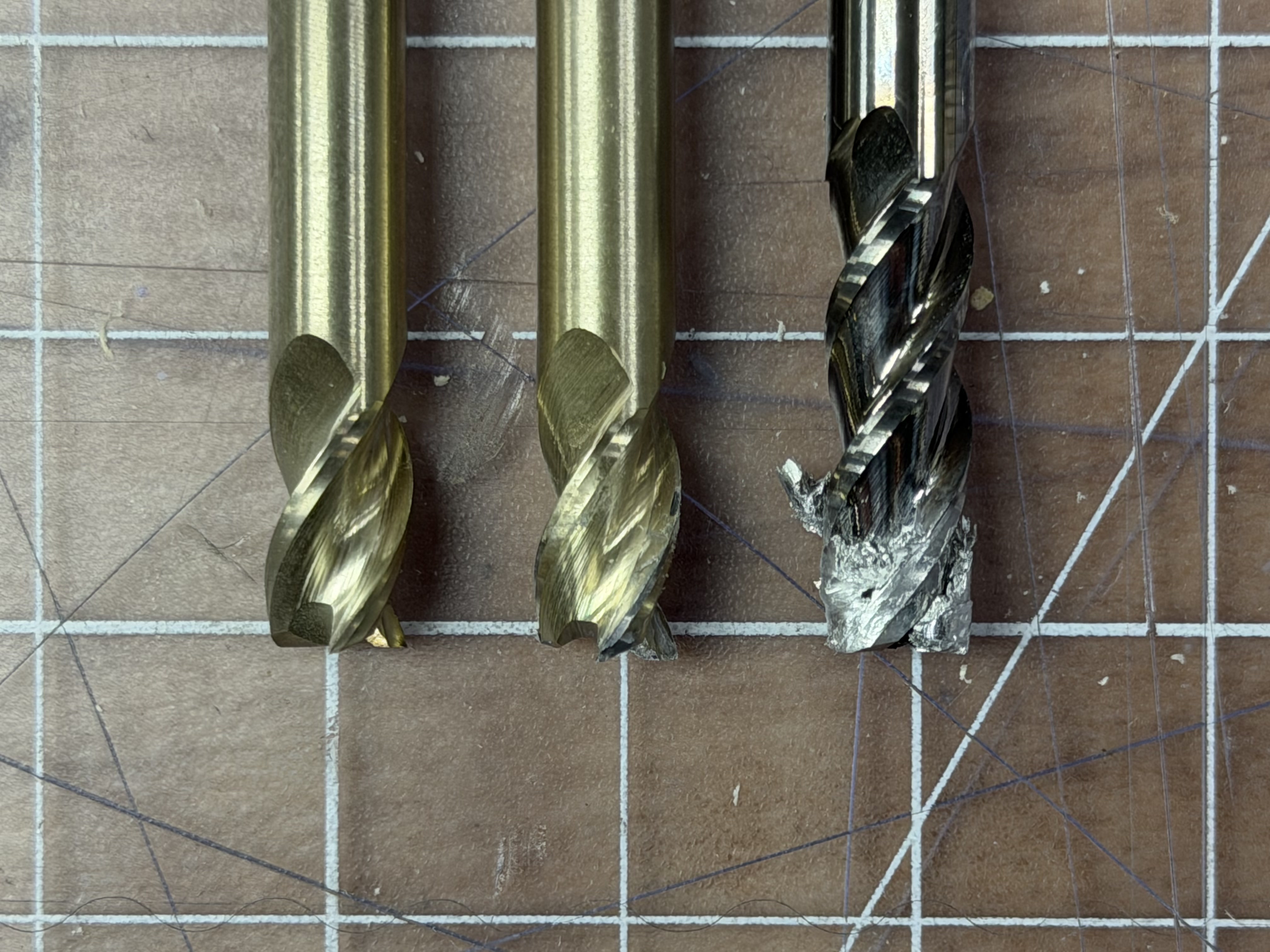
Machining the same toolpath and target velocities using a trapezoidal velocity planner (left),
vs the model-based velocity solver (right).
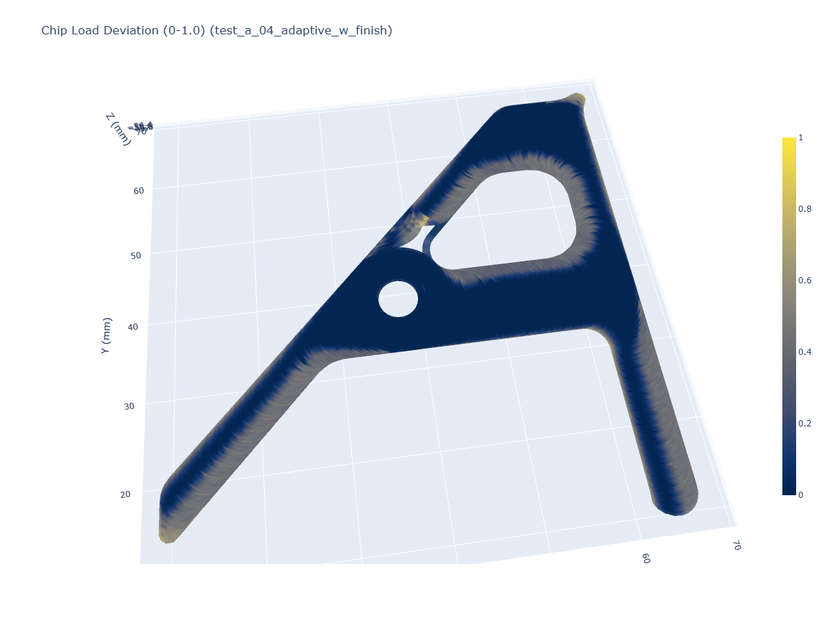
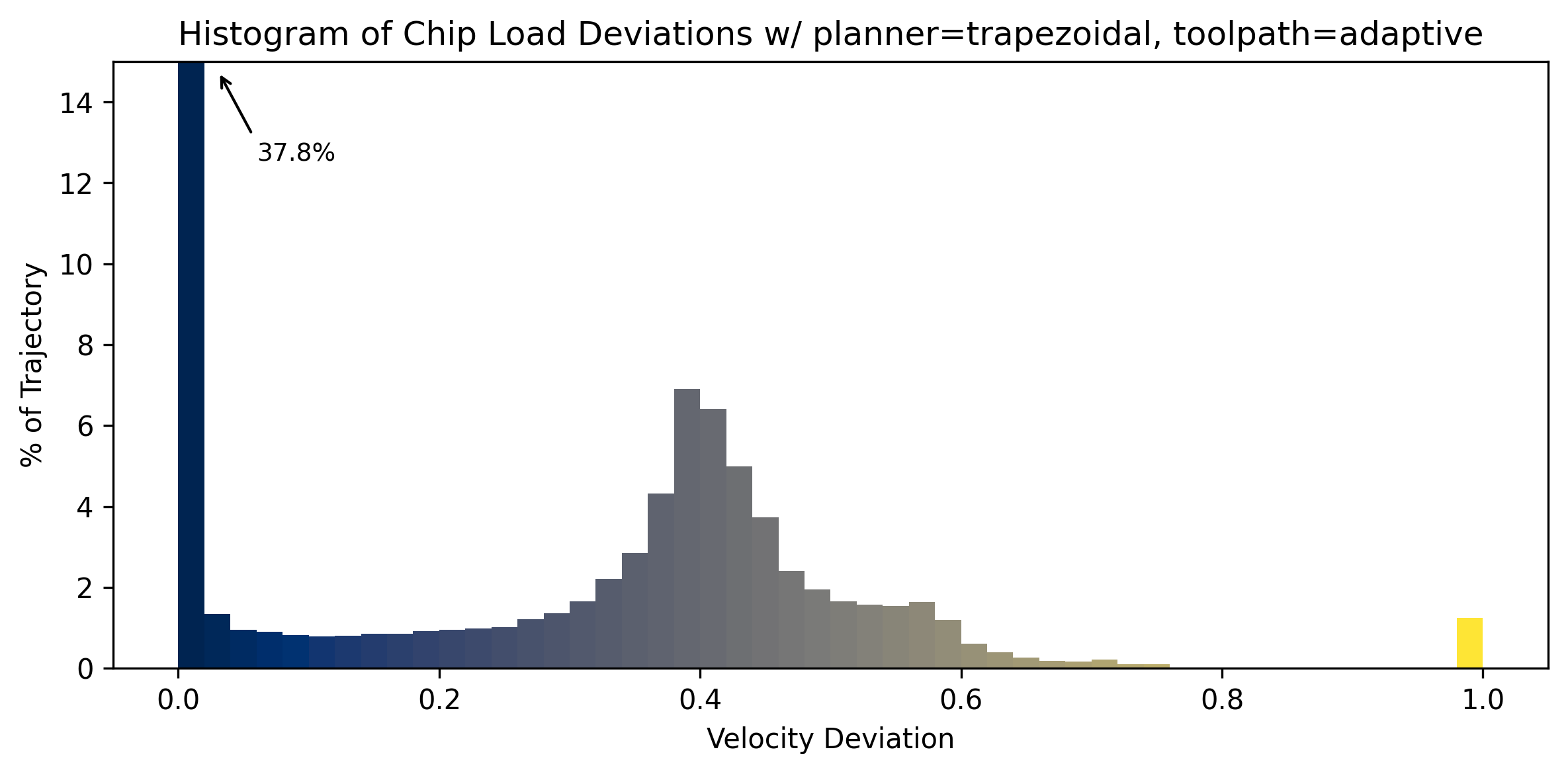
Chip load deviations, trapezoid solver.
(blue good, yellow bad).
(blue good, yellow bad).
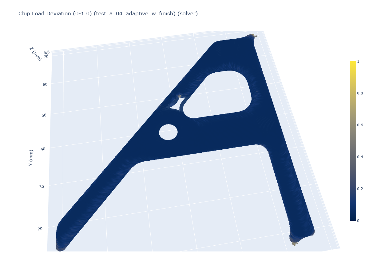
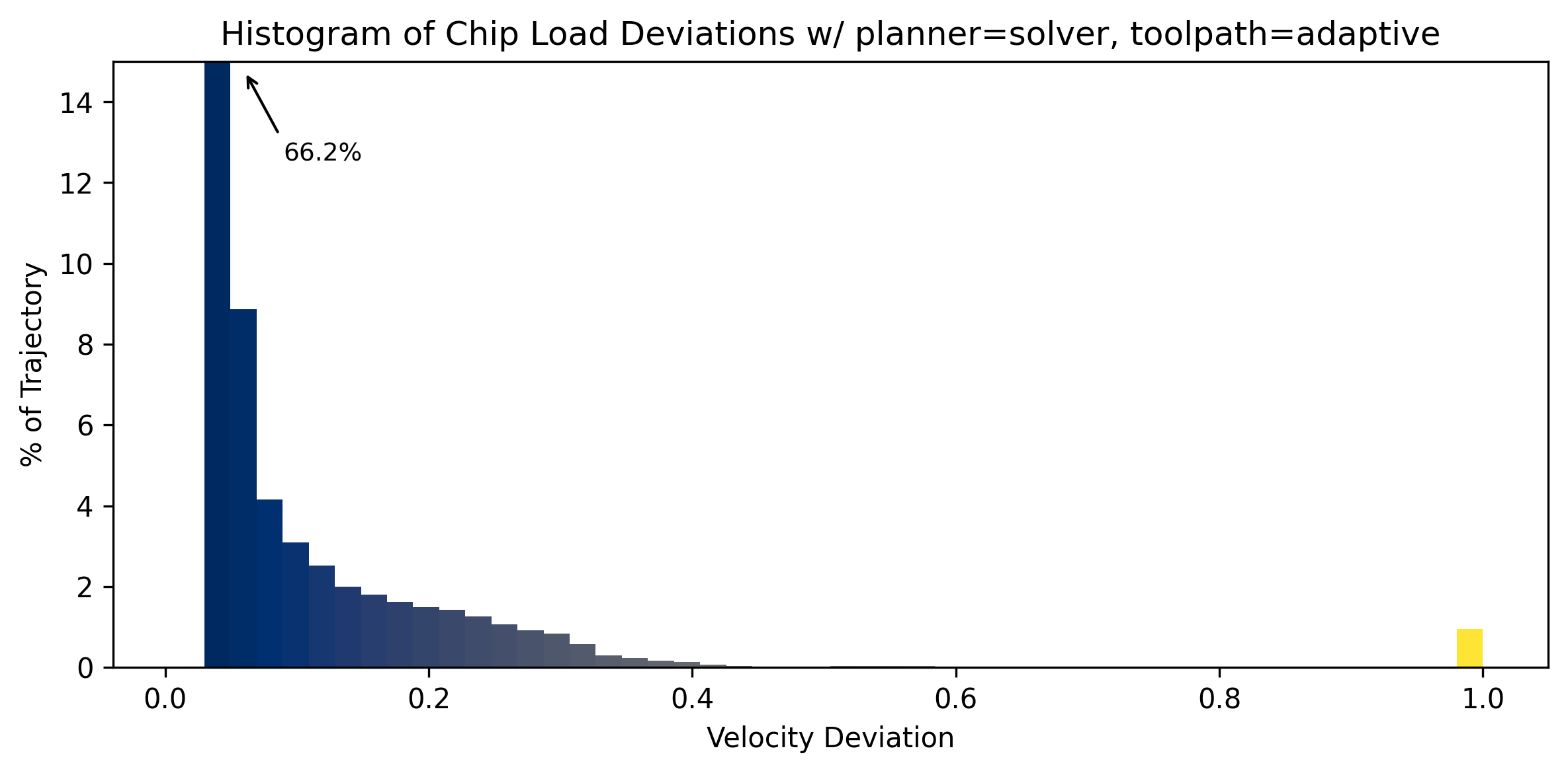
Chip load deviations, model-based solver.
(blue good, yellow bad).
(blue good, yellow bad).
Framing velocity control as an explicit constrained optimization problem
leads to performance improvements that can have meaningful impact on process outcomes.
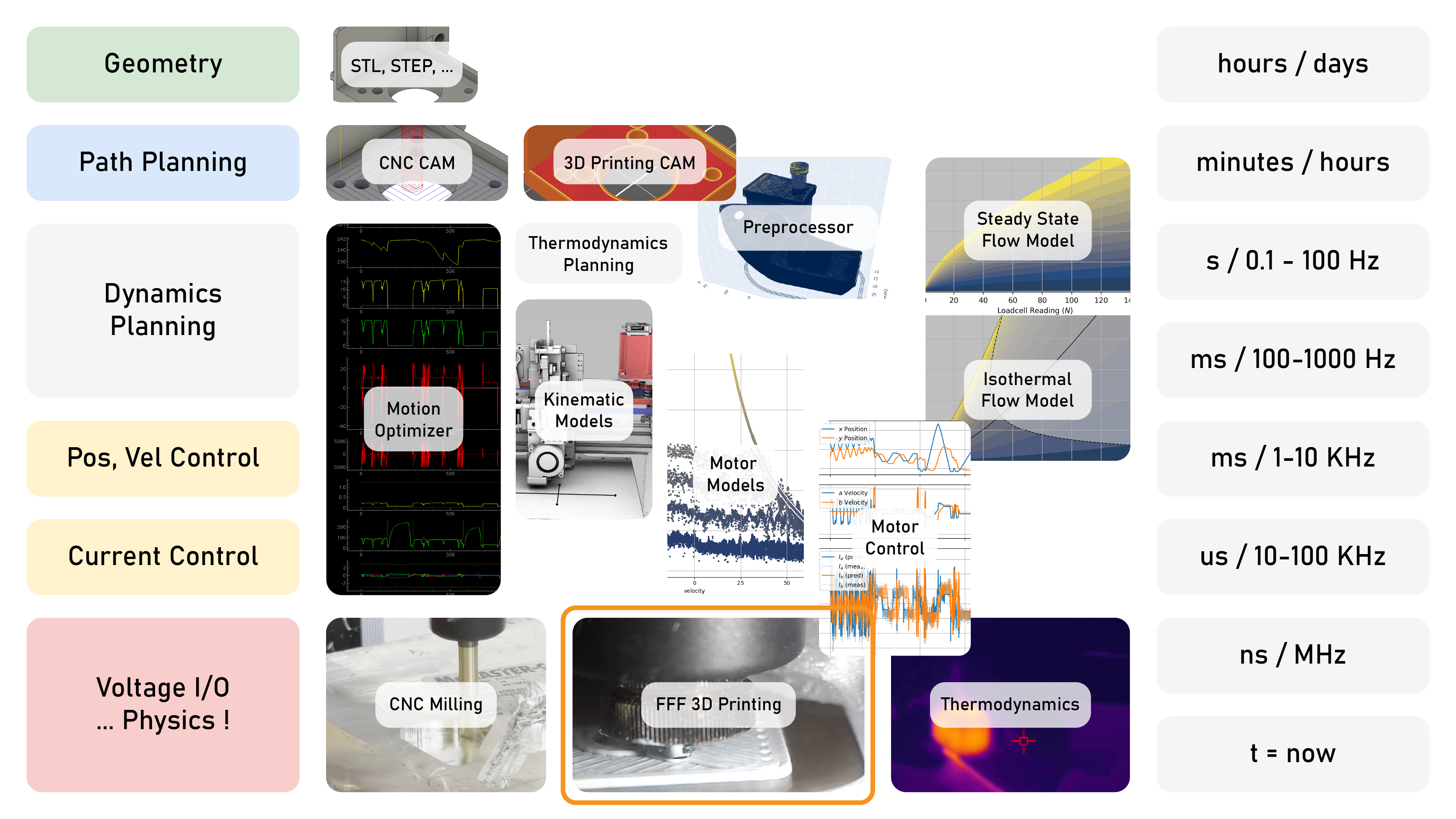
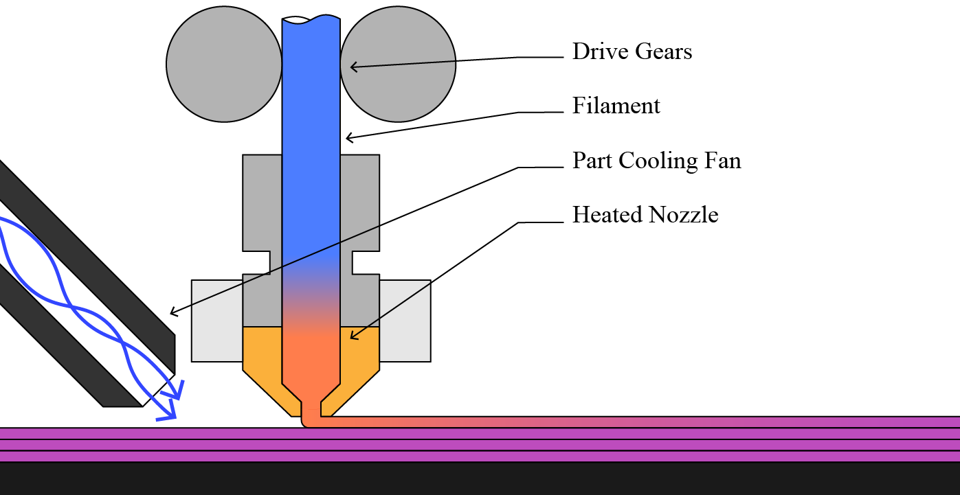
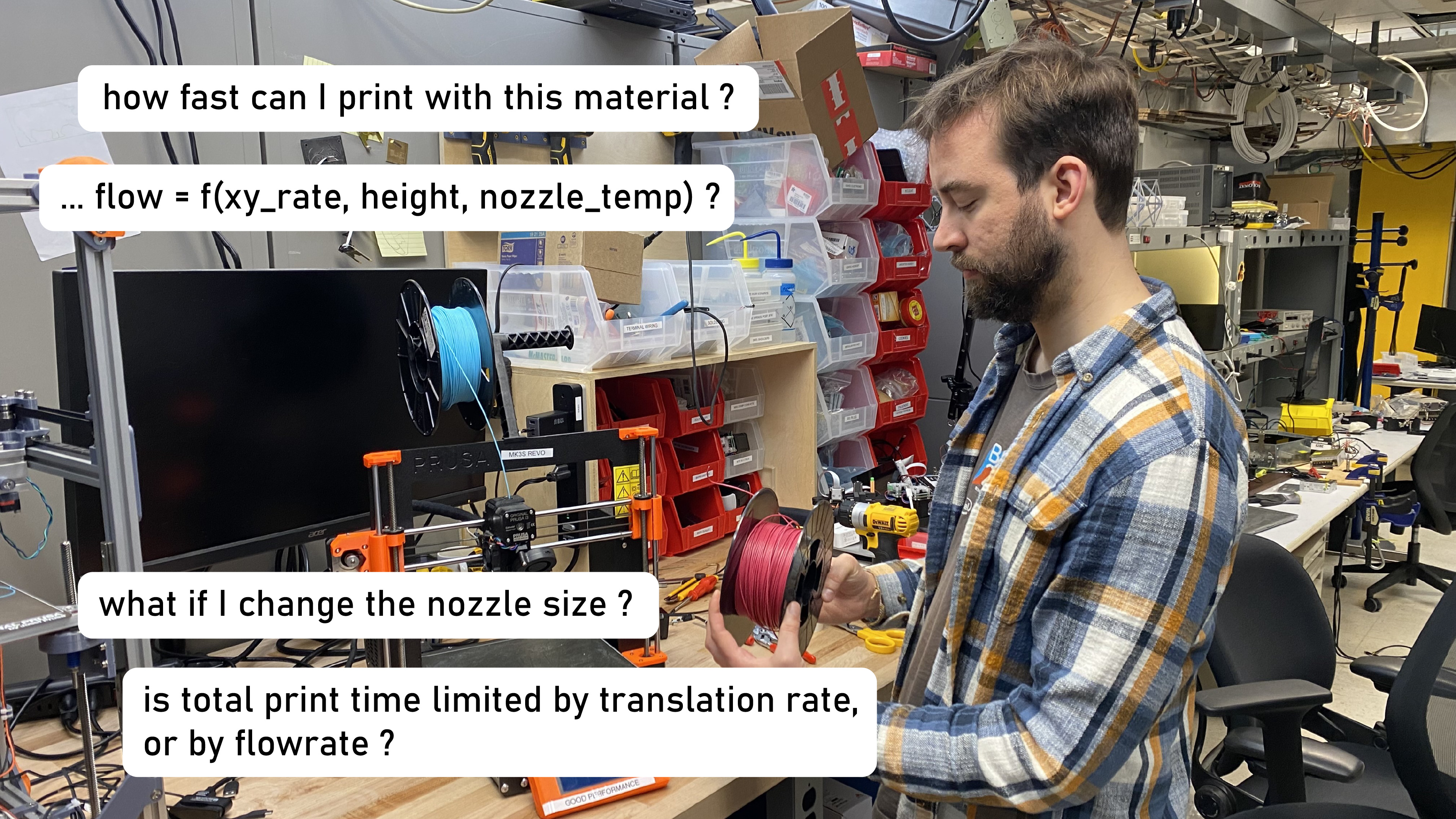
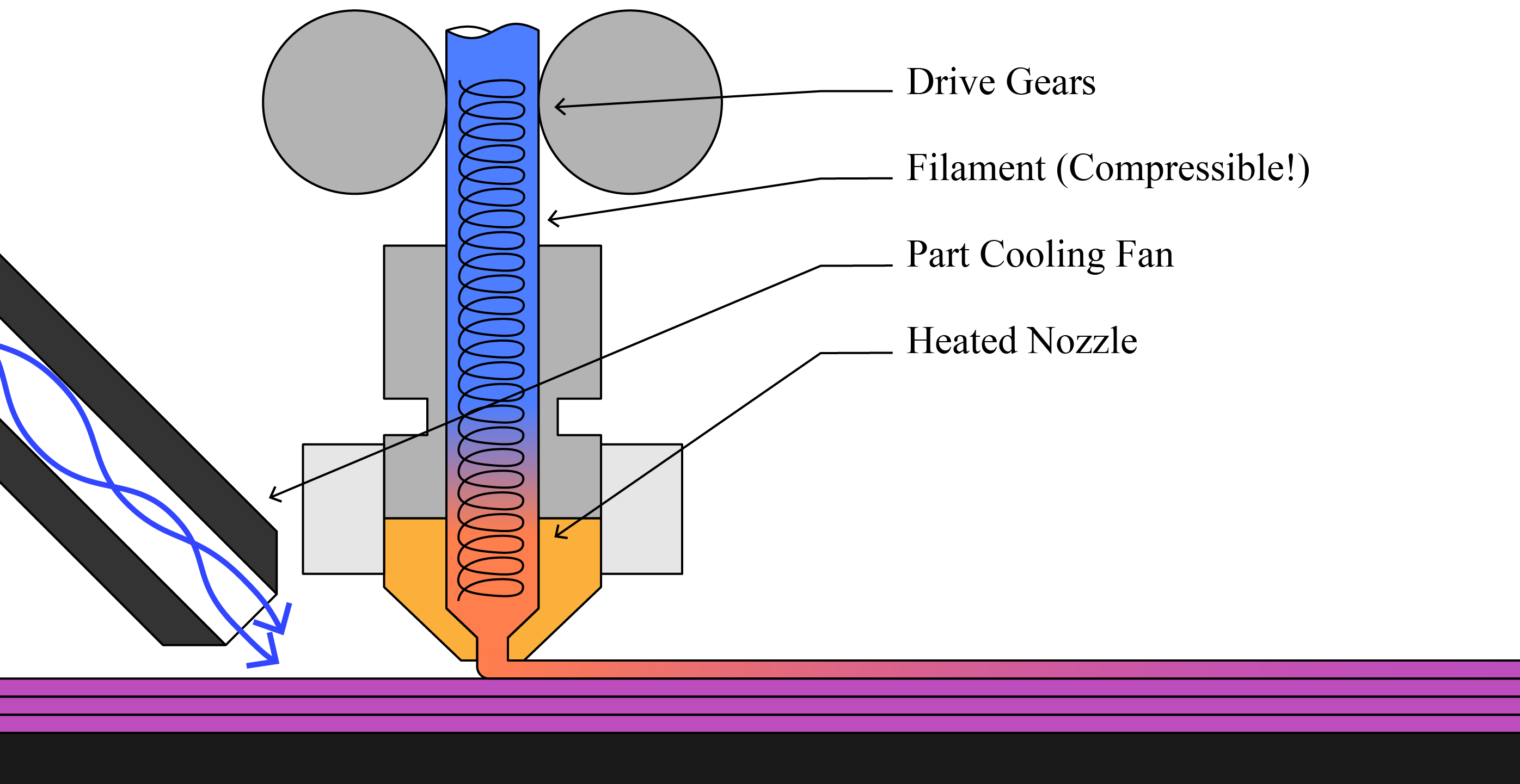
Heat, squish, and extrude a thermopolymer through a nozzle.
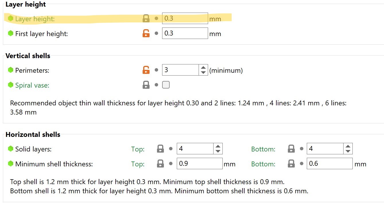
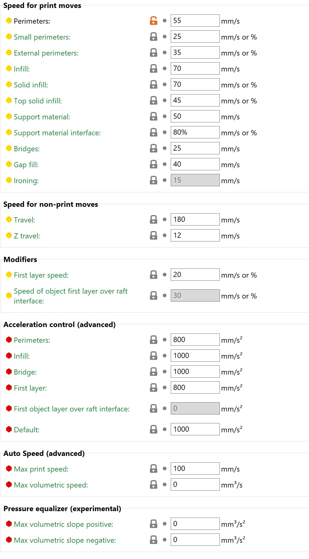
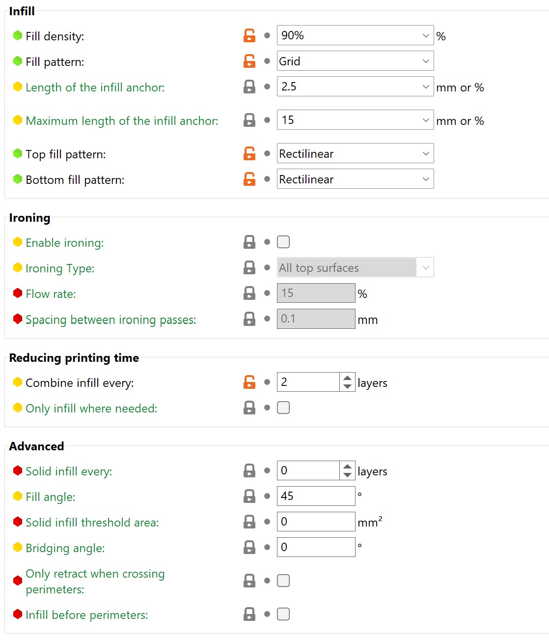
3D printing Parameters as shown to users in PrusaSlicer
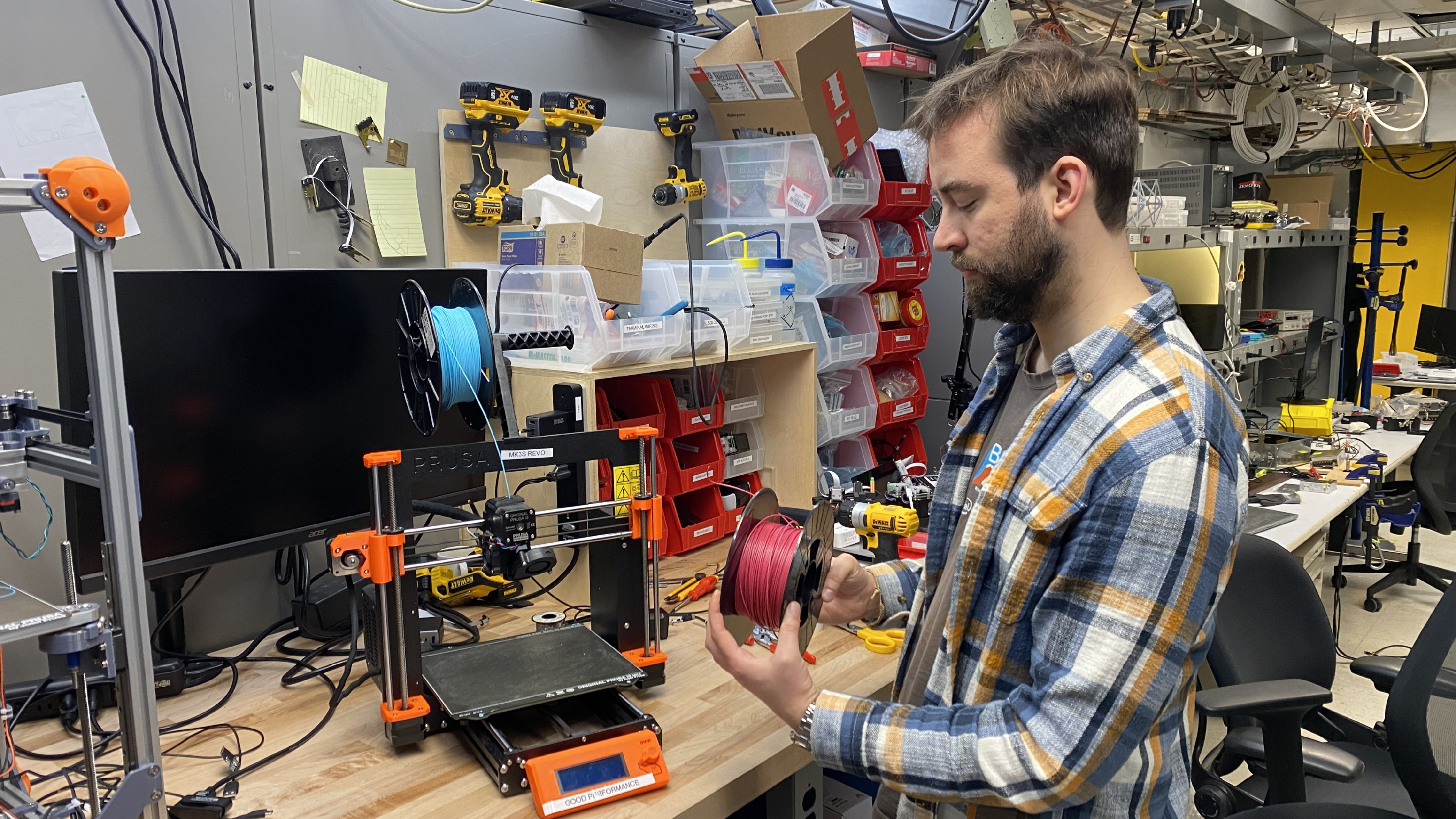
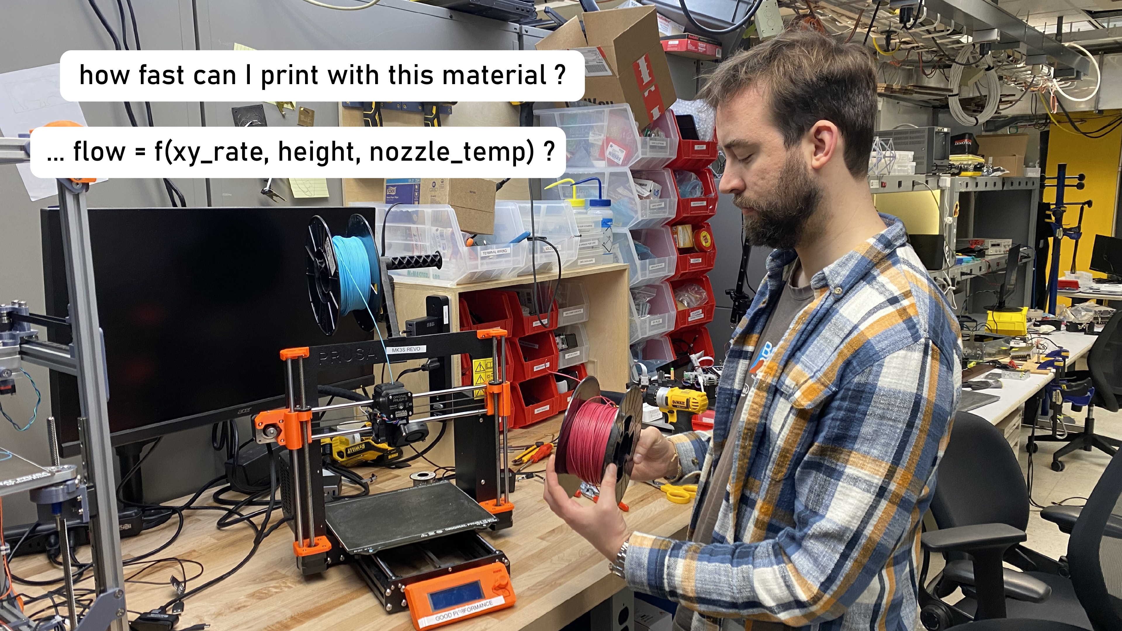
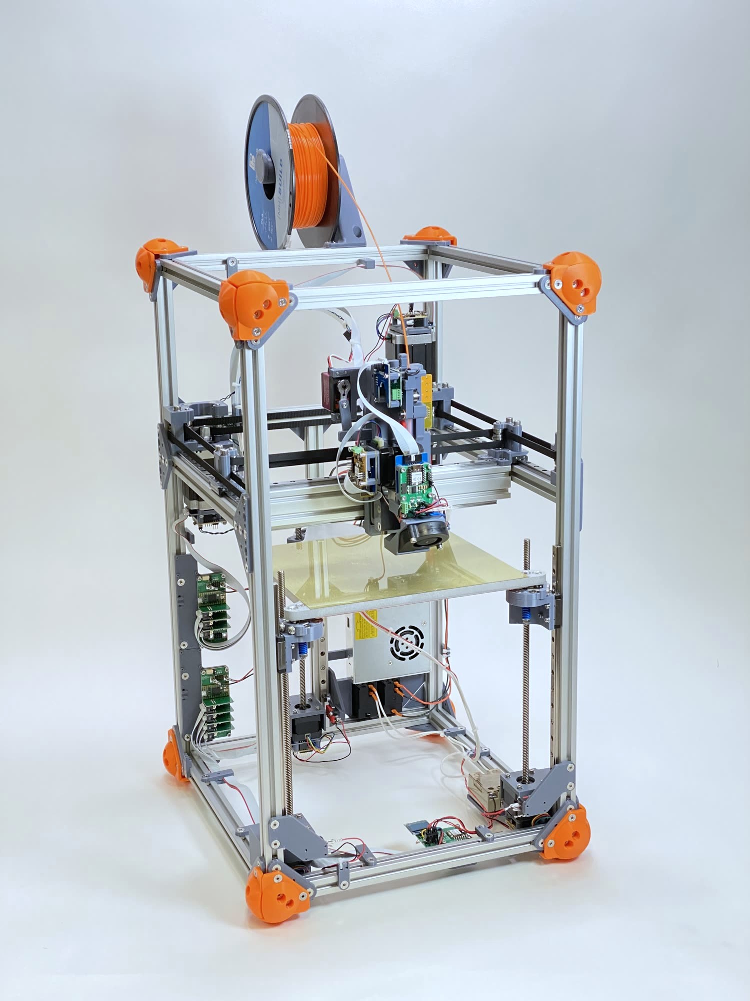
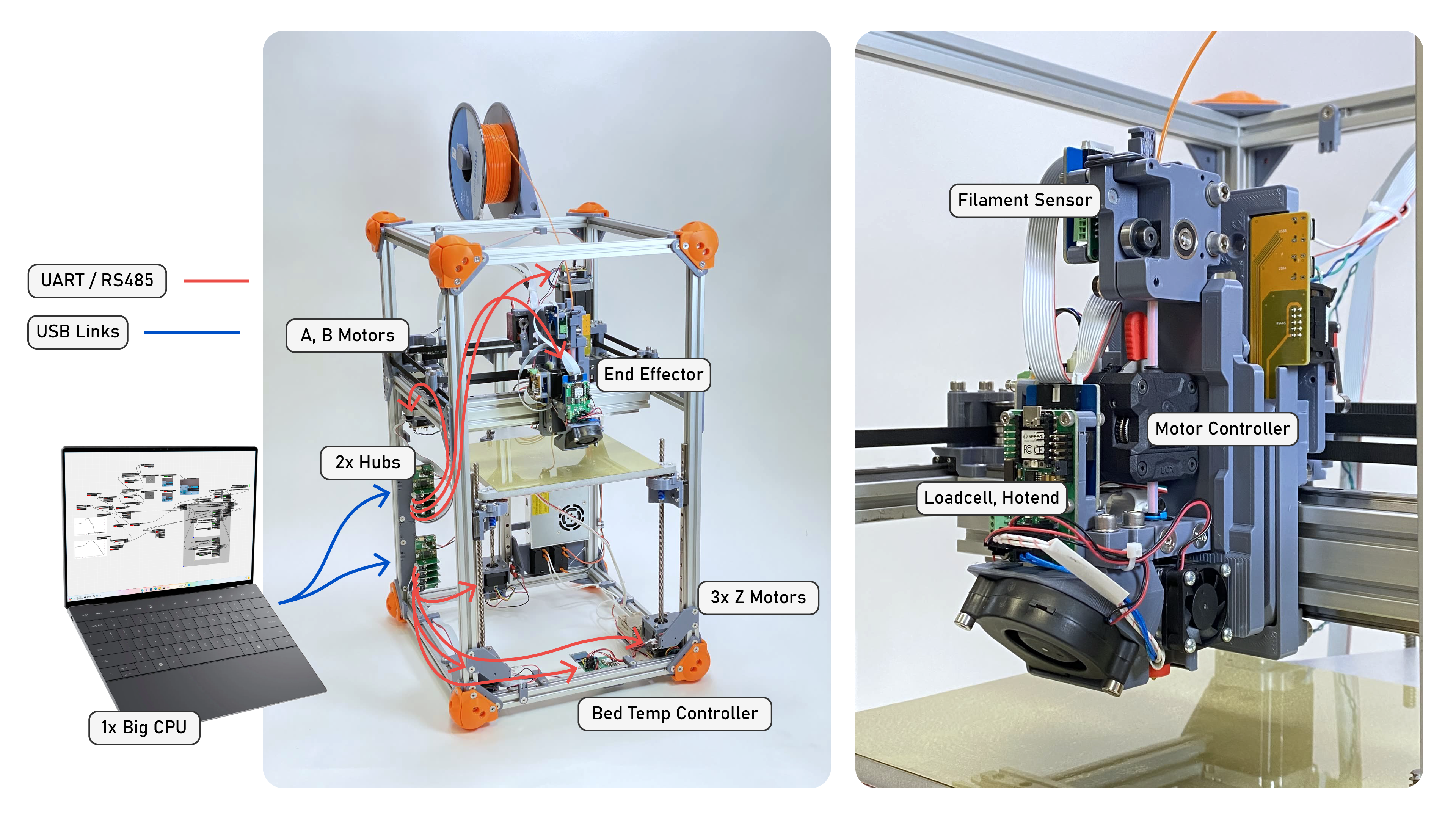
The RheoPrinter
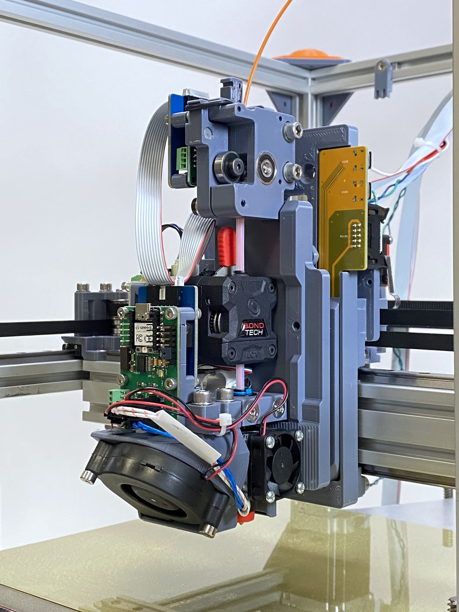
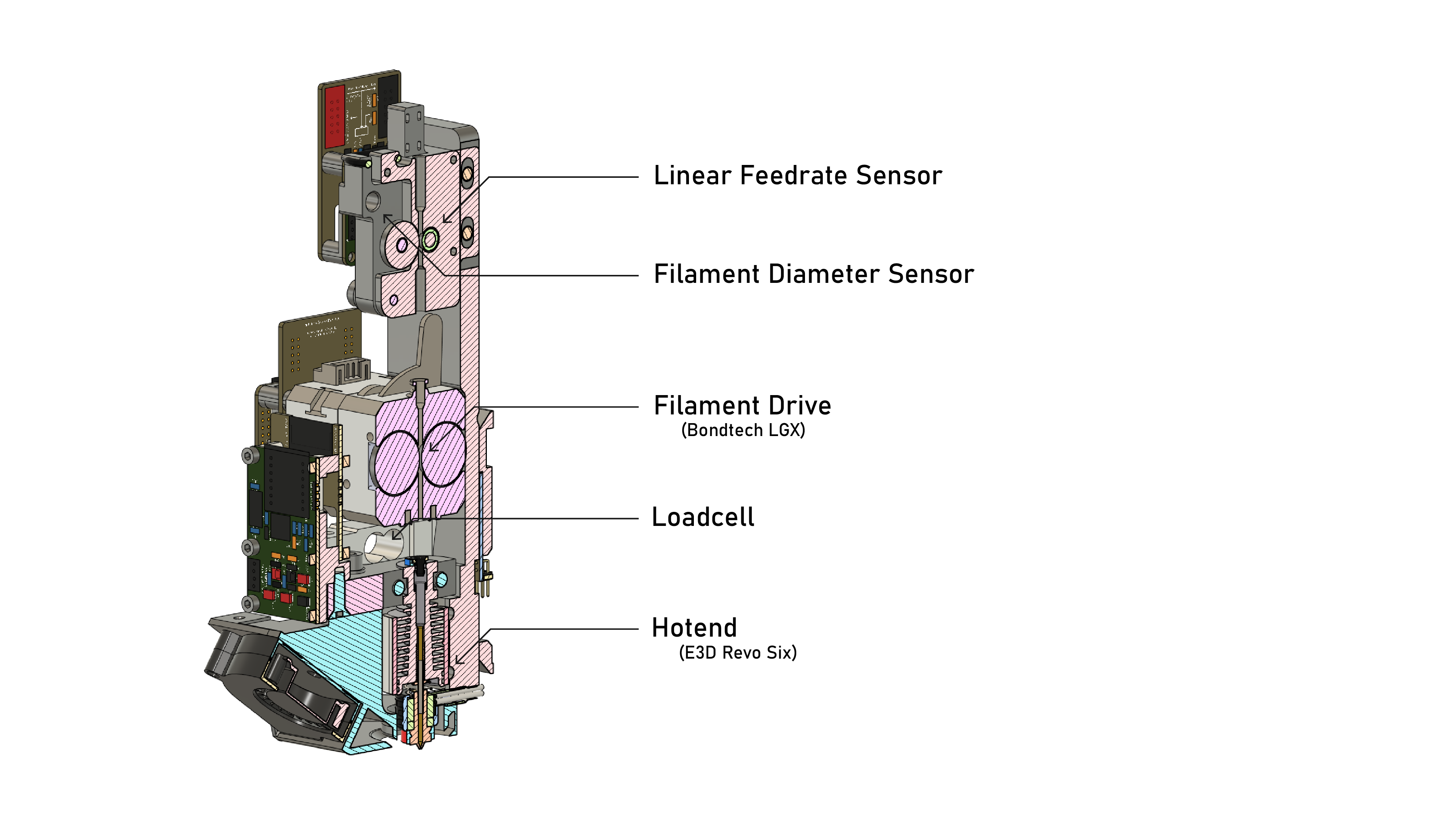
The RheoPrinter's Extruder
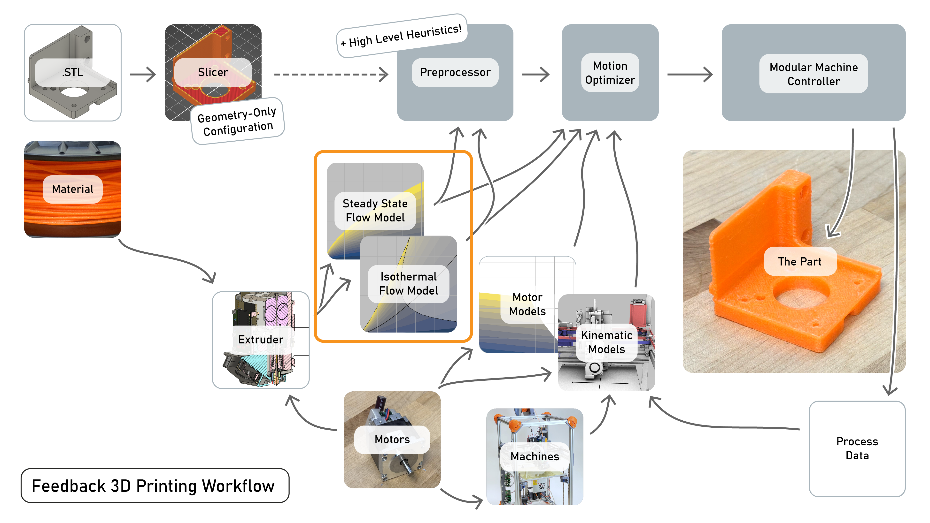
Steady-State Flow Model
In steady-state:
For any temperature, what flowrates are possible?
What is the pressure required for each?
For any temperature, what flowrates are possible?
What is the pressure required for each?
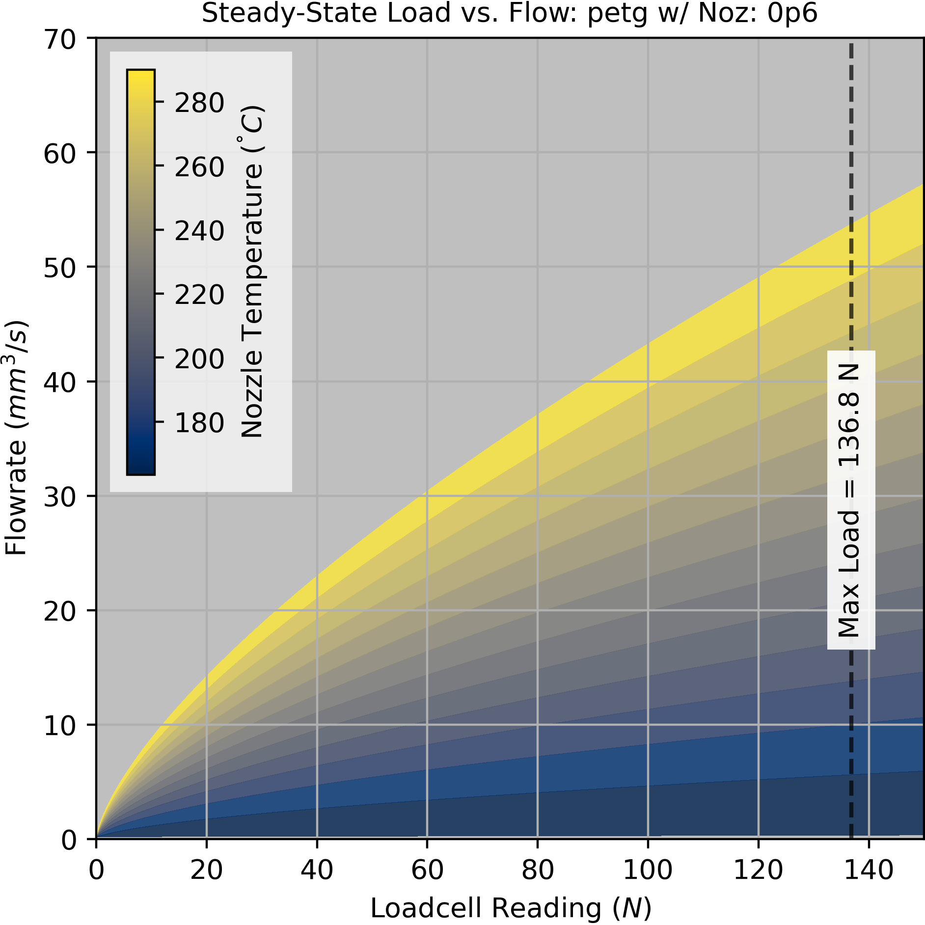
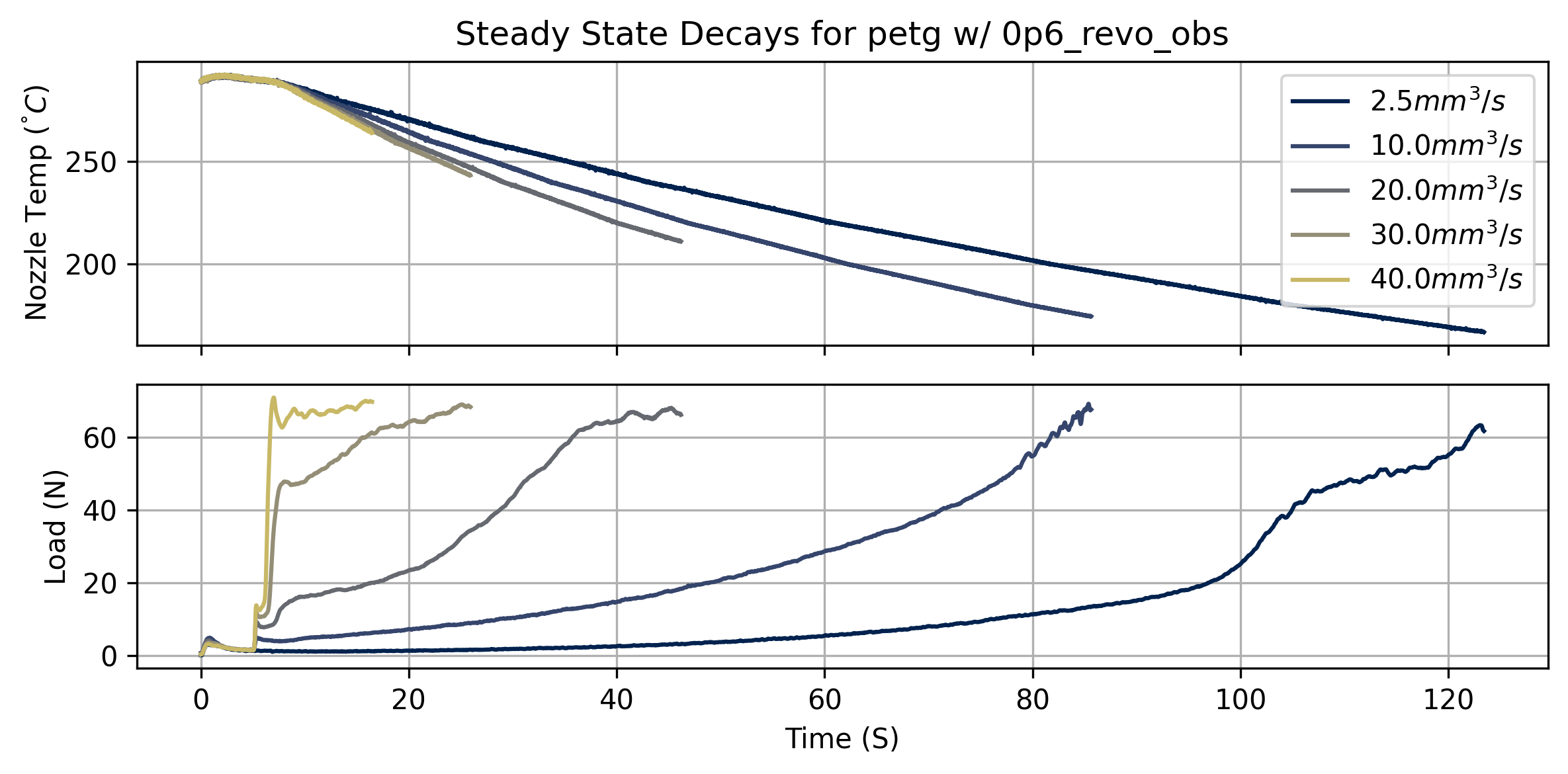
For a range of flowrates:
- Heat the nozzle to its maximum temperature.
- Set the extruder to drive at the test flowrate.
- Disable the heater!
- Until the flow stops, record:
- Nozzle temperature,
- Extruder motor current,
- Loadcell pressure,
- Continue to next test flowrate.
$$
Q = f(Fk_{lin}) ^ {k_{pow}}
$$
$Q (mm^3/s)$ is volumetric flowrate.
$F (N)$ is the loadcell reading.
$k_{lin}, k_{pow}$ are temperature-varying parameters.
$F (N)$ is the loadcell reading.
$k_{lin}, k_{pow}$ are temperature-varying parameters.
$$
\begin{aligned}
k_{lin} &= T_{norm} a_{ss} + b_{ss} \\
k_{pow} &= T_{norm} c_{ss} + d_{ss} \\
\end{aligned}
$$
| Symbol | Value | Units | Source |
| --- | --- | ---: | :--- |
| $Q_{ss}$ | Volmetric Flowrate | $mm^3/s$ | Motor |
| $F$ | Nozzle Load | $N$ | Loadcell |
| $T$ | Temperature of Flow | $^\\degree C$ | Measured |
| $T_{norm}$ | Normalized Temp. | | $\left( \frac{T - T_{min}}{T_{max} - T_{min}} \right)$ |
| $T_{max}$ | Maximum Temp. for Flow | $^\\degree C$ | Nozzle / Heater Limit |
| $T_{min}$ | Minimum Temp. for Flow | $^\\degree C$ | **Fit in this step.** |
| $k_{lin}$ | Flow Linear Term | n/a | $f(a_{ss}, b_{ss}, T_{min})$ |
| $k_{pow}$ | Flow Power Term | n/a | $f(c_{ss}, d_{ss}, T_{min})$ |
| $a_{ss}$ | Model Parameter | n/a | Model Fit |
| $b_{ss}$ | Model Parameter | n/a | Model Fit |
| $c_{ss}$ | Model Parameter | n/a | Model Fit |
| $d_{ss}$ | Model Parameter | n/a | Model Fit |
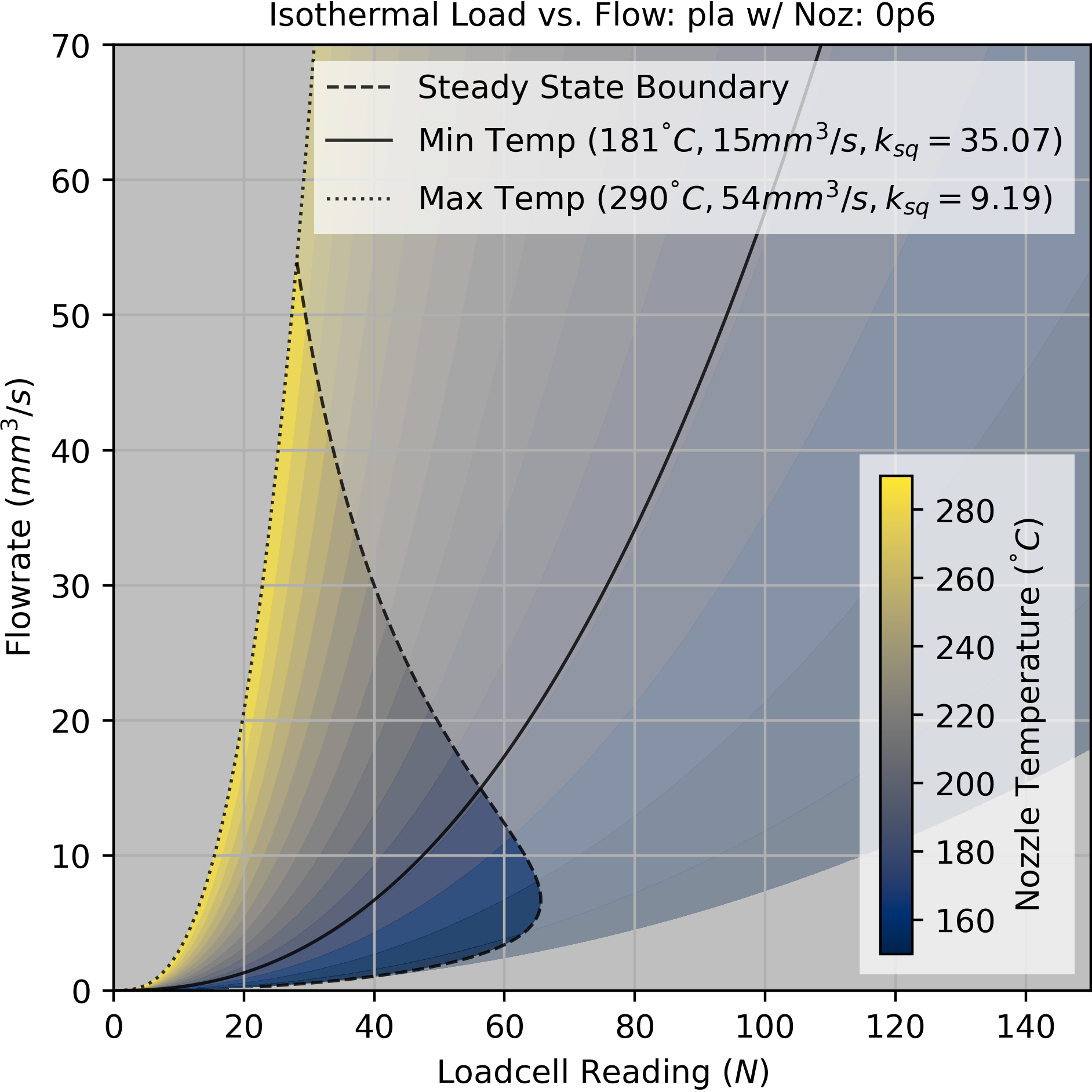
Isothermal Flow Model
Over short time-scales:
For any temperature and pressure, what flowrate should we expect?
At each temperature, how compressible is the filament?
For any temperature and pressure, what flowrate should we expect?
At each temperature, how compressible is the filament?
For a range of temperatures:
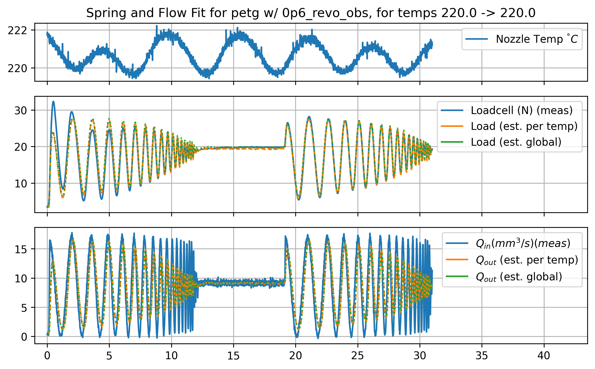
- Heat to the test temperature
- Run a chirp test with changing extruder motor speeds.
- Record:
- Nozzle temperature,
- Extruder motor current,
- Loadcell pressure,
- Continue to next test temperature.
$$
\begin{aligned}
Q_{out} &= f(F \cdot k_{lin}) ^ {k_{pow}} \\
\Delta F &= (Q_{in} - Q_{out})k_{sq} \\
\end{aligned}
$$
We now have two volumetric flowrates $(mm^3/s)$:
$F (N)$ is the loadcell reading.
$k_{lin}, k_{pow}, k_{sq}$ are temperature-varying parameters.
- $Q_{in} $ into the melt-zone,
- $Q_{out}$ out from the nozzle.
$F (N)$ is the loadcell reading.
$k_{lin}, k_{pow}, k_{sq}$ are temperature-varying parameters.
$$
\begin{aligned}
k_{lin} &= T_{norm} a_{iso} + b_{iso} \\
k_{pow} &= T_{norm} c_{iso} + d_{iso} \\
k_{sq} &= T_{norm} k_{sq,a} + k_{sq,b} \\
\end{aligned}
$$
| Symbol | Value | Units | Source |
| --- | --- | ---: | :--- |
| $Q_{in}$ | Flowrate **into the heater** | $mm^3/s$ | Measured |
| $Q_{out}$ | Flowrate **at nozzle** | $mm^3/s$ | Estimated |
| $F$ | Nozzle Load | $N$ | Loadcell |
| $T$ | Temperature of Flow | $^\\degree C$ | Measured |
| $T_{norm}$ | Normalized Temp. | | $\left( \frac{T - T_{min}}{T_{max} - T_{min}} \right)$ |
| $T_{max}$ | Maximum Temp. for Flow | $^\\degree C$ | Nozzle / Heater Limit |
| $T_{min}$ | Minimum Temp. for Flow | $^\\degree C$ | **Via steady-state fit** |
| $k_{lin}$ | Flow Linear Term | n/a | $f(a_{iso}, b_{iso}, T_{min})$ |
| $k_{pow}$ | Flow Power Term | n/a | $f(c_{iso}, d_{iso}, T_{min})$ |
| $k_{sq}$ | **Filament Springrate** | $N/mm^3$ | Model Fit |
| $a_{iso}$ | Model Parameter | n/a | Model Fit |
| $b_{iso}$ | Model Parameter | n/a | Model Fit |
| $c_{iso}$ | Model Parameter | n/a | Model Fit |
| $d_{iso}$ | Model Parameter | n/a | Model Fit |
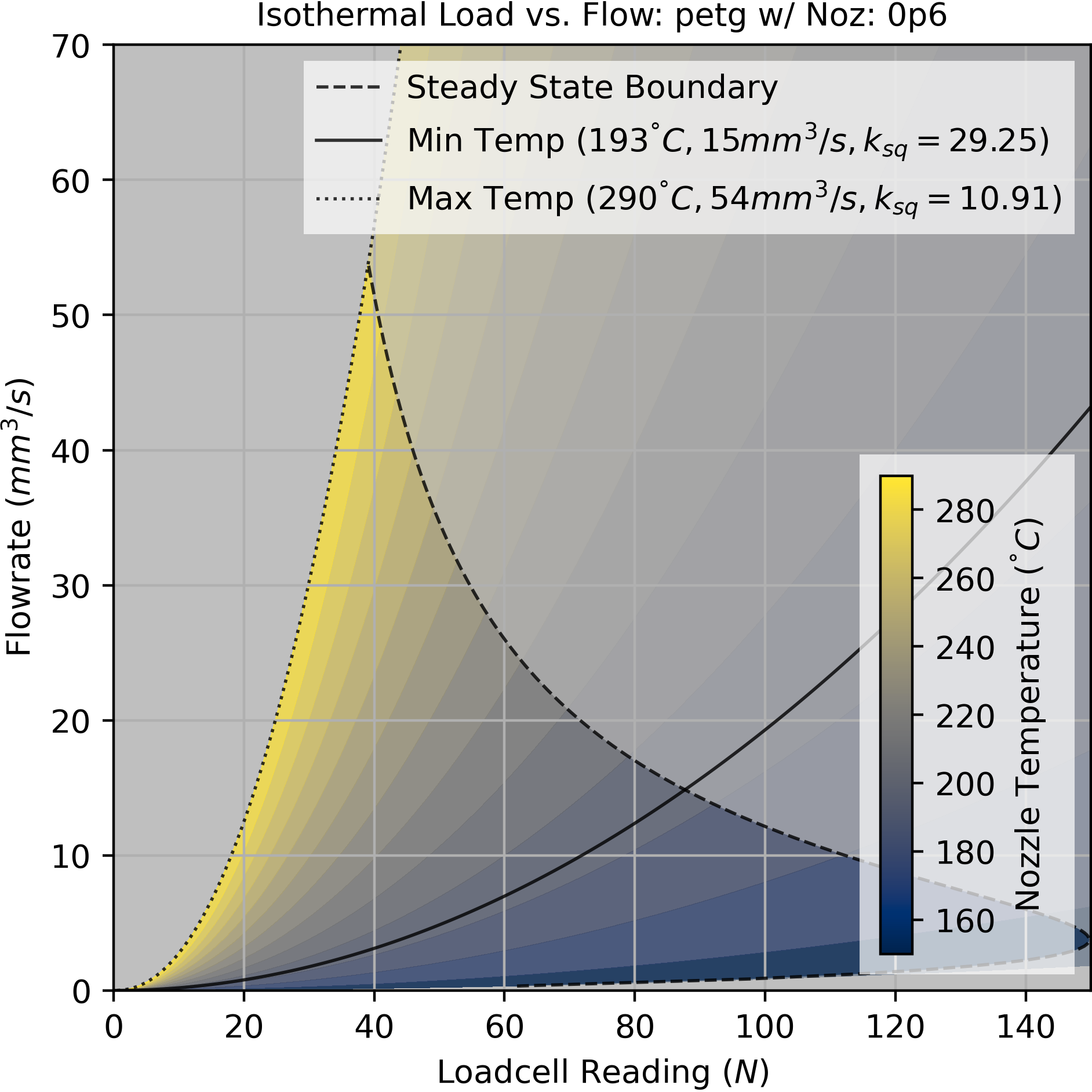
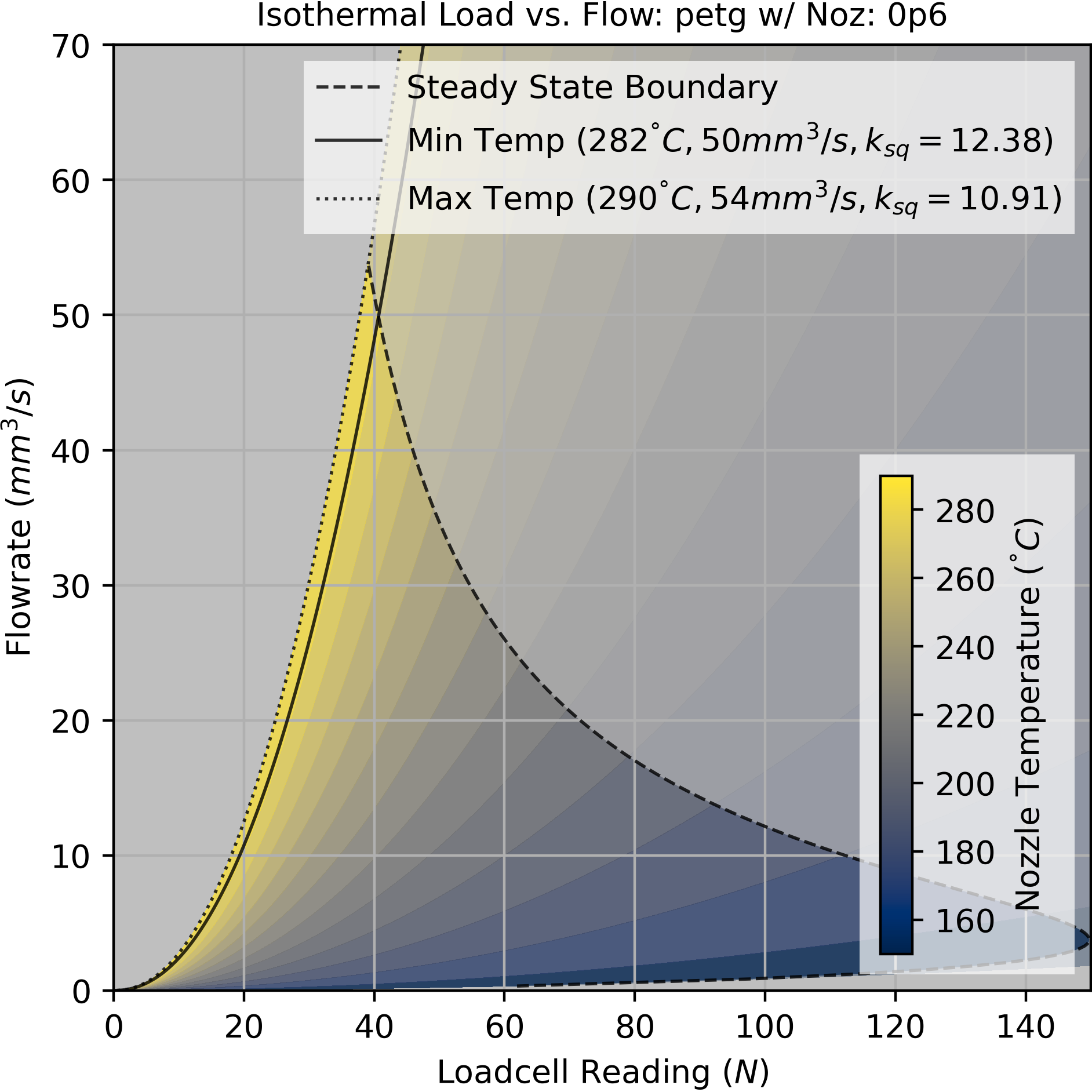
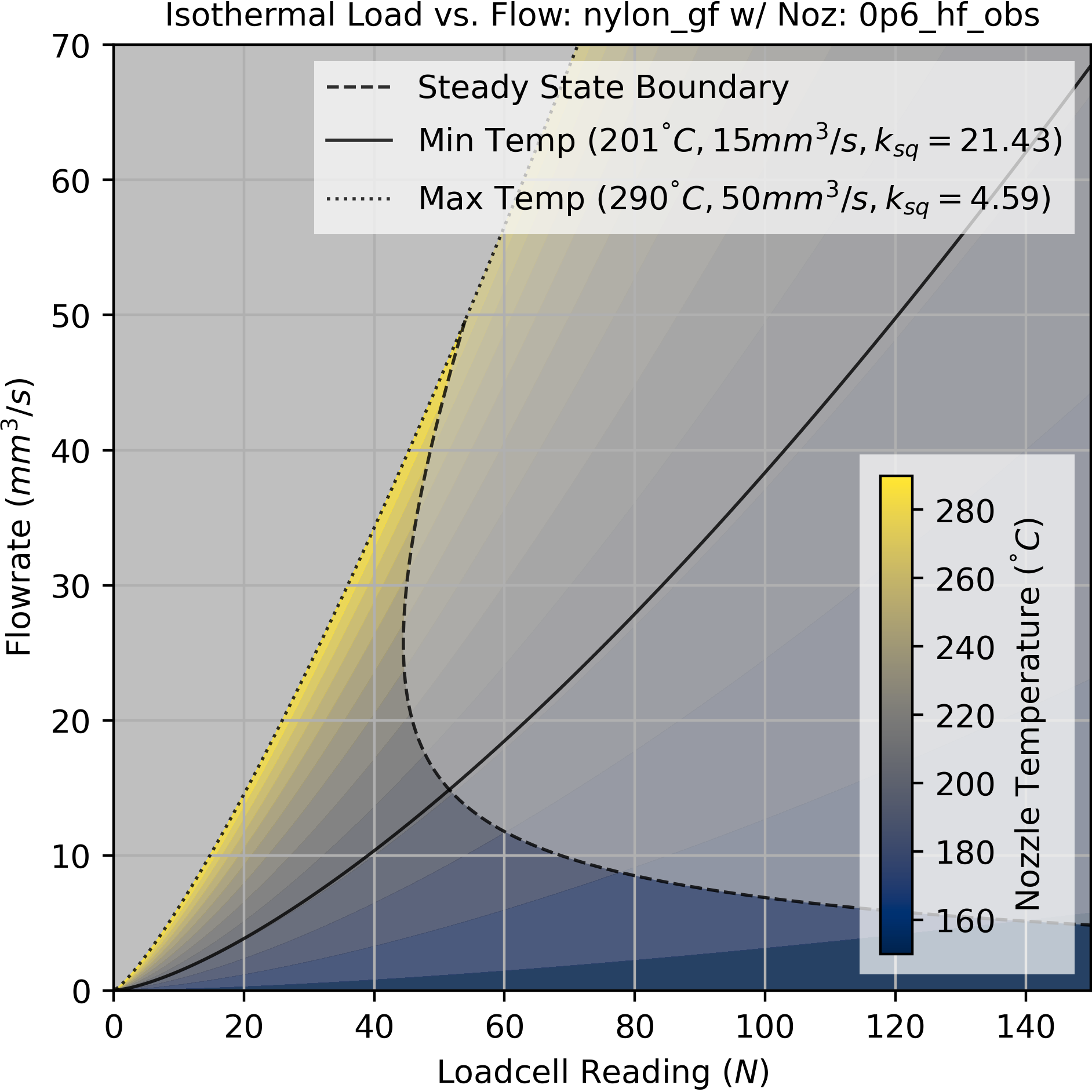
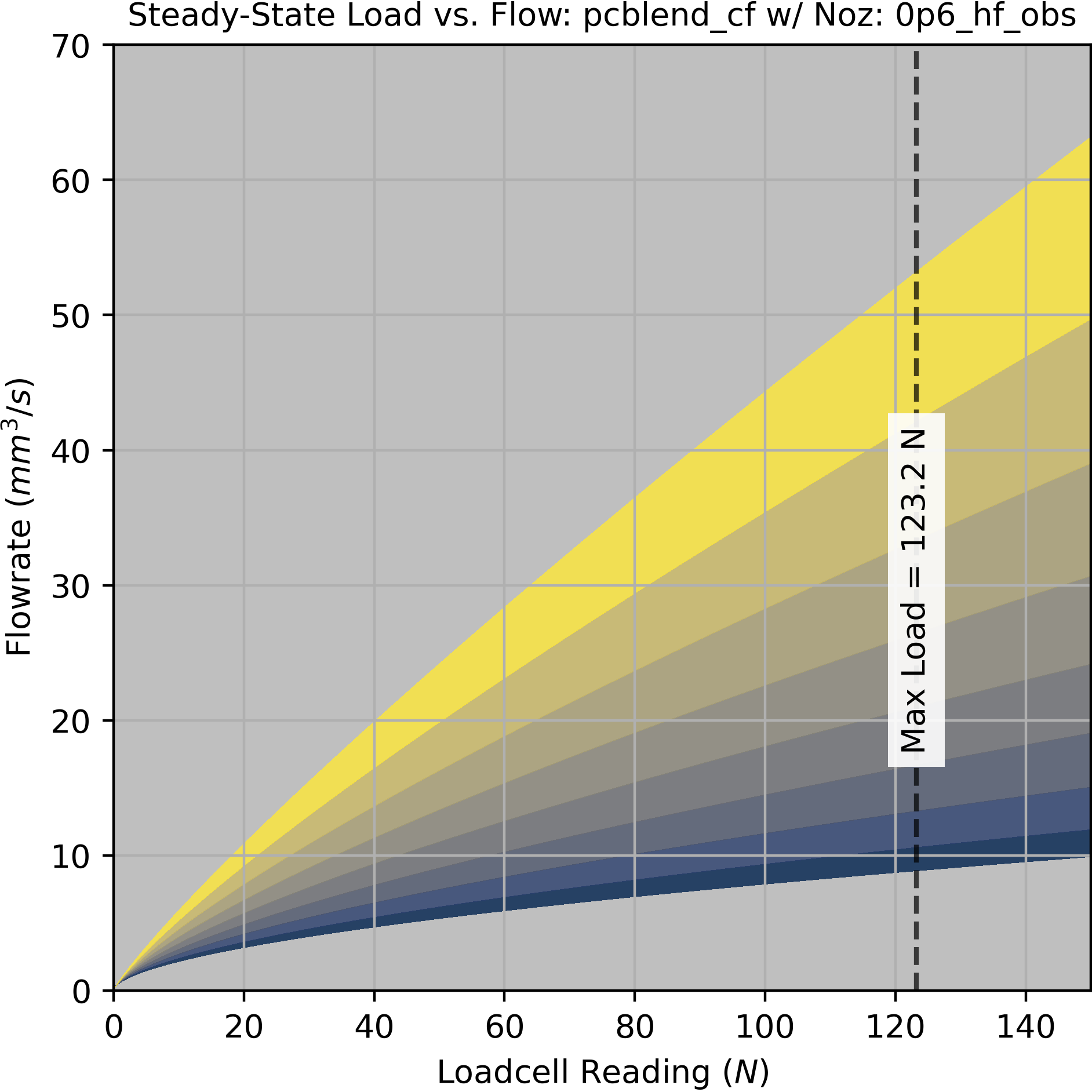
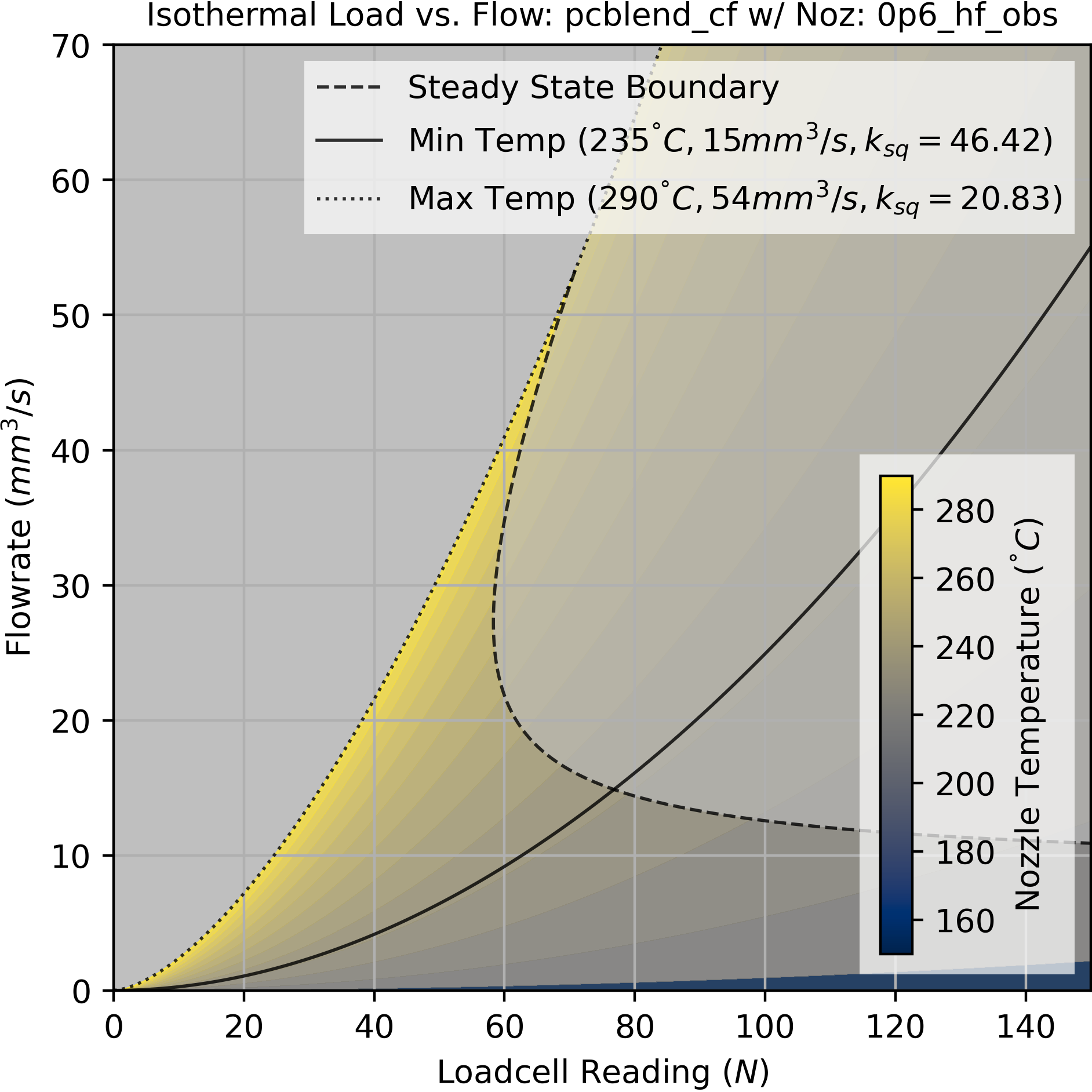
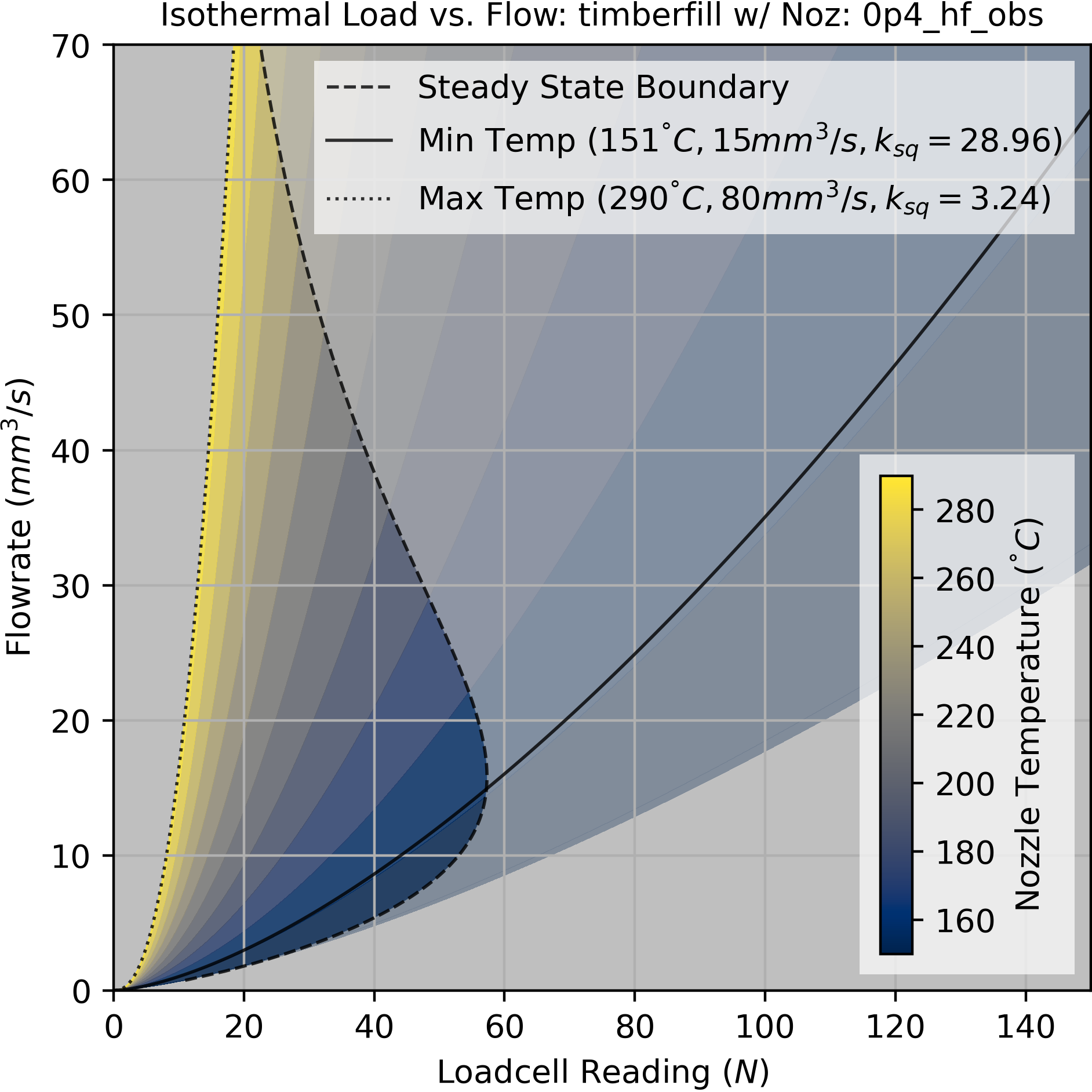
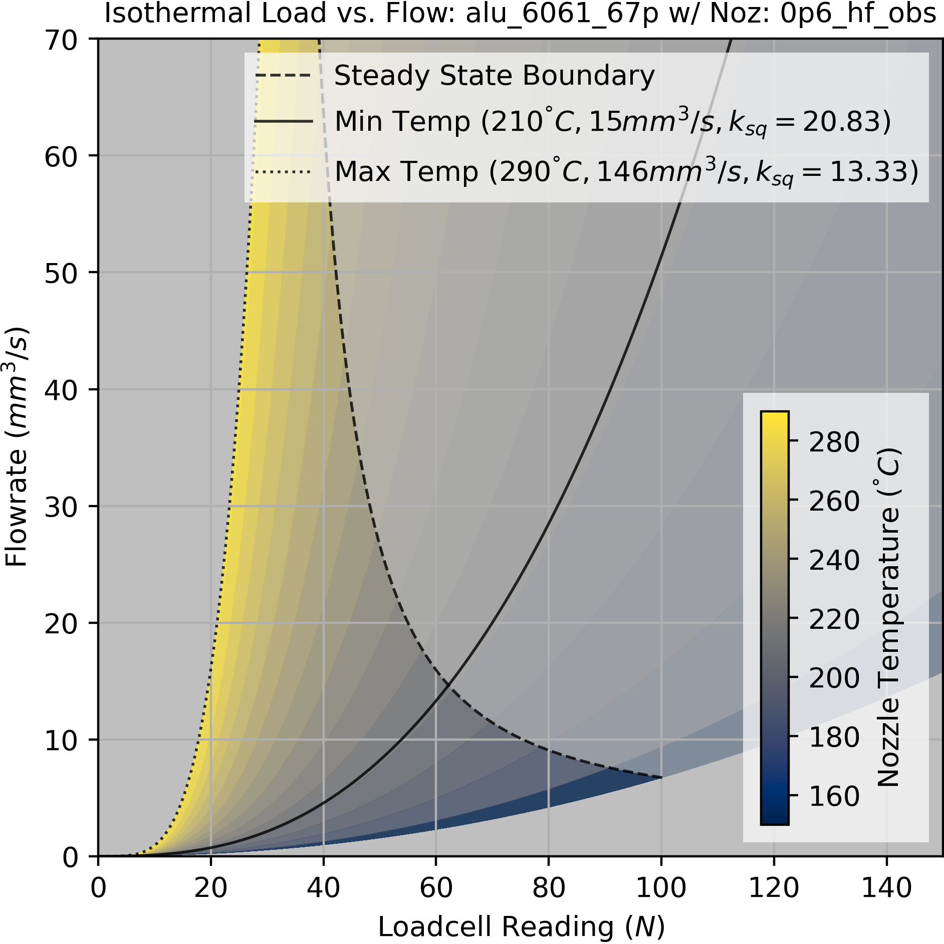
Models to the right characterize PETG (Polyethylene Terephthalate Glycol) filament, w/ 0.6mm Nozzle.
$\text{Flowrate} \ Q = f(F \cdot k_{lin}) ^ {k_{pow}}$
The steady-state model shows decreasing flowrate at higher loads, due to nozzle heating losses.
$k_{pow} < 1.0$
The isothermal model shows increasing flowrate at higher loads, because of shear thinning.
$k_{pow} > 1.0$
* The steady state boundary is a projection of the steady-state model onto the isothermal model.
The steady-state model characterizes long term phenomenology.
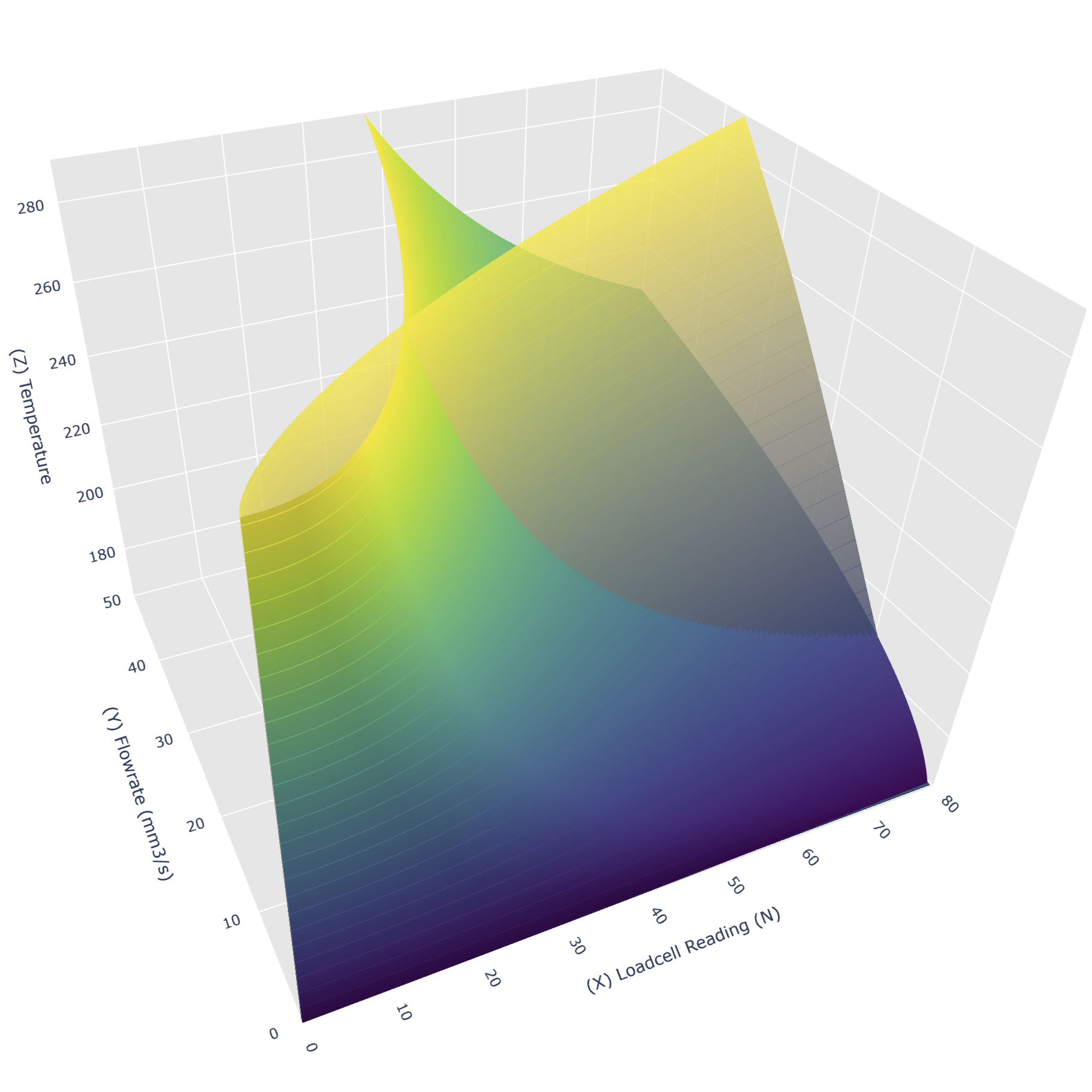
Models diverge at high flowrates, where
melt flow temperature != nozzle temperature
melt flow temperature != nozzle temperature
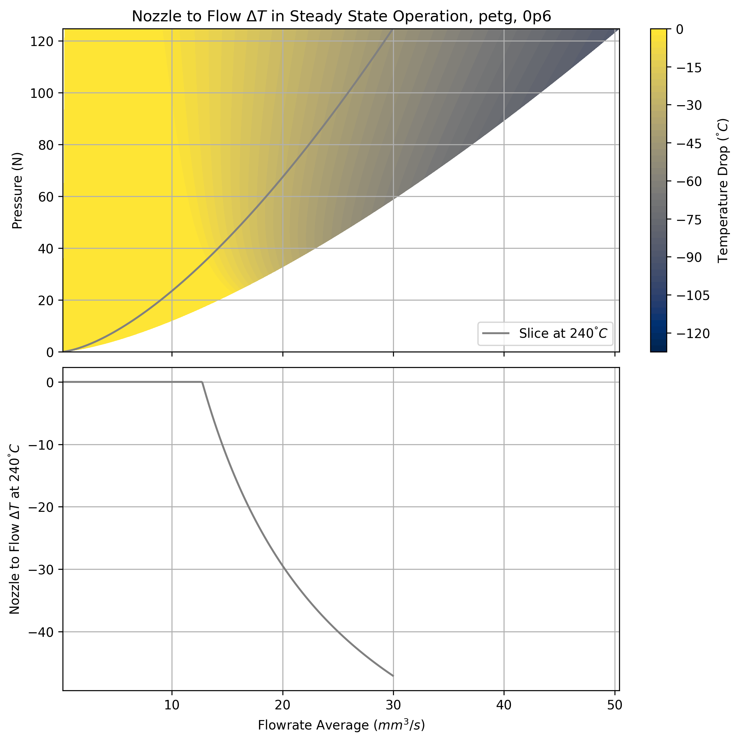
Taking a slice at a chosen nozzle temperature
divergence = $\Delta T$ at any average flowrate.
divergence = $\Delta T$ at any average flowrate.
The isothermal model characterizes "instantaneous" phenomenology.
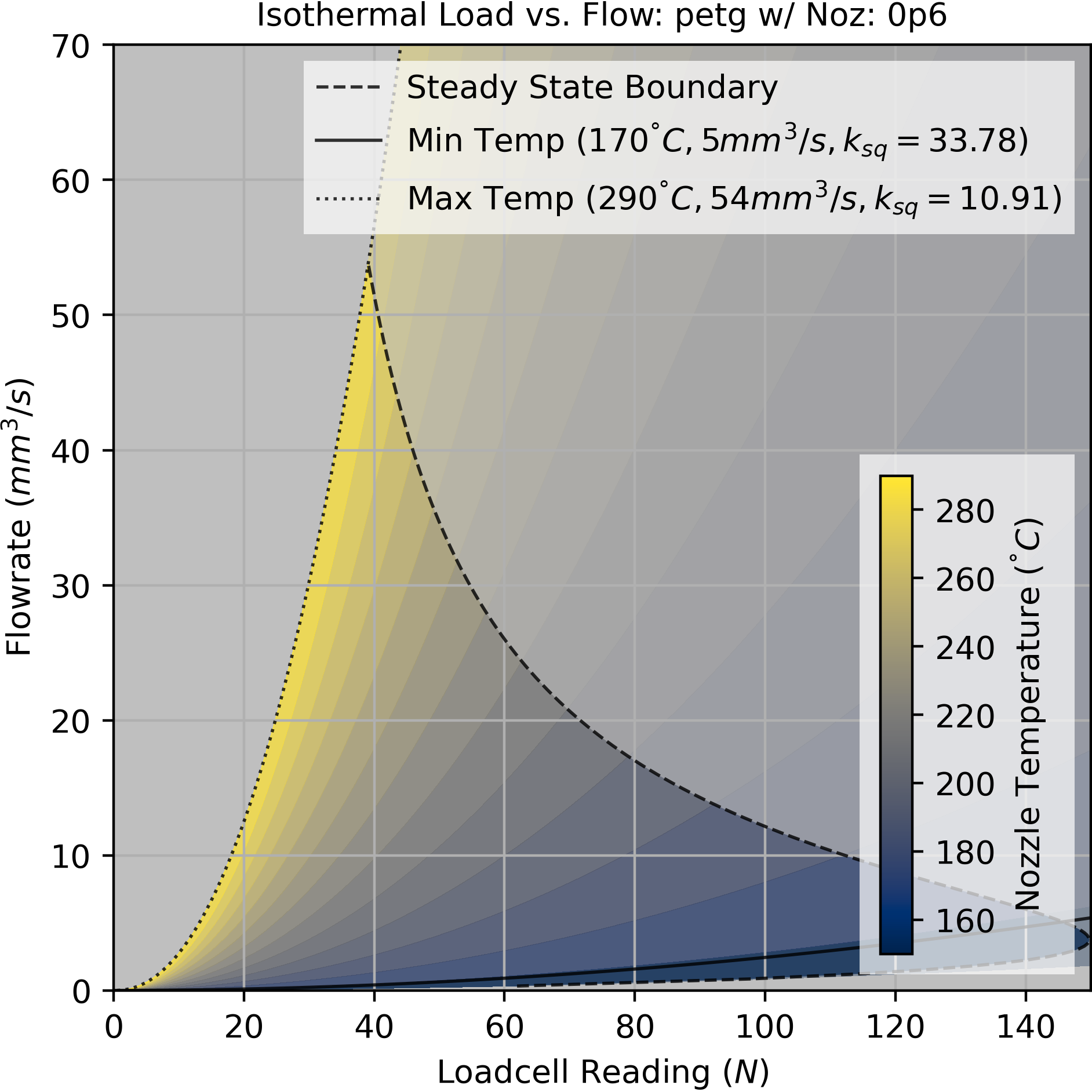
Any temperature and flowrate within this boundary is possible,
How do we pick the optimal set?
How do we pick the optimal set?
Start with temperature, which we can select using minimum flow.
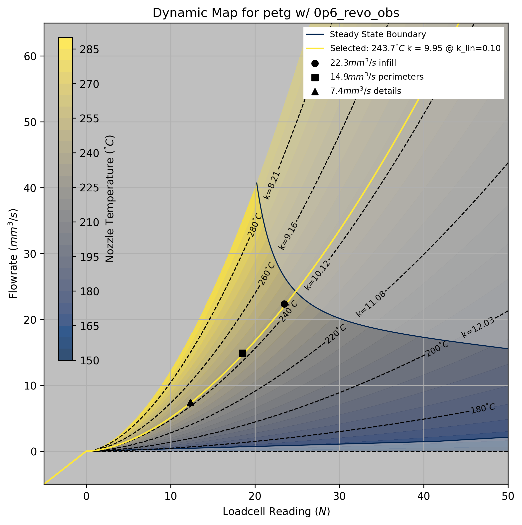
Another heuristic to pick flowrates:
use higher pressures during infill and
lower during perimeters and detailed parts of the print.
We can use our machine's own hardware to make rheological models.
We can mix heuristics with models, to combine tacit knowledge
with real-world constraints to broadcast intuition across our systems' heterogeneity.
So, can we also formulate higher-level optimizations, i.e. for time optimality? (fast good, slow bad)
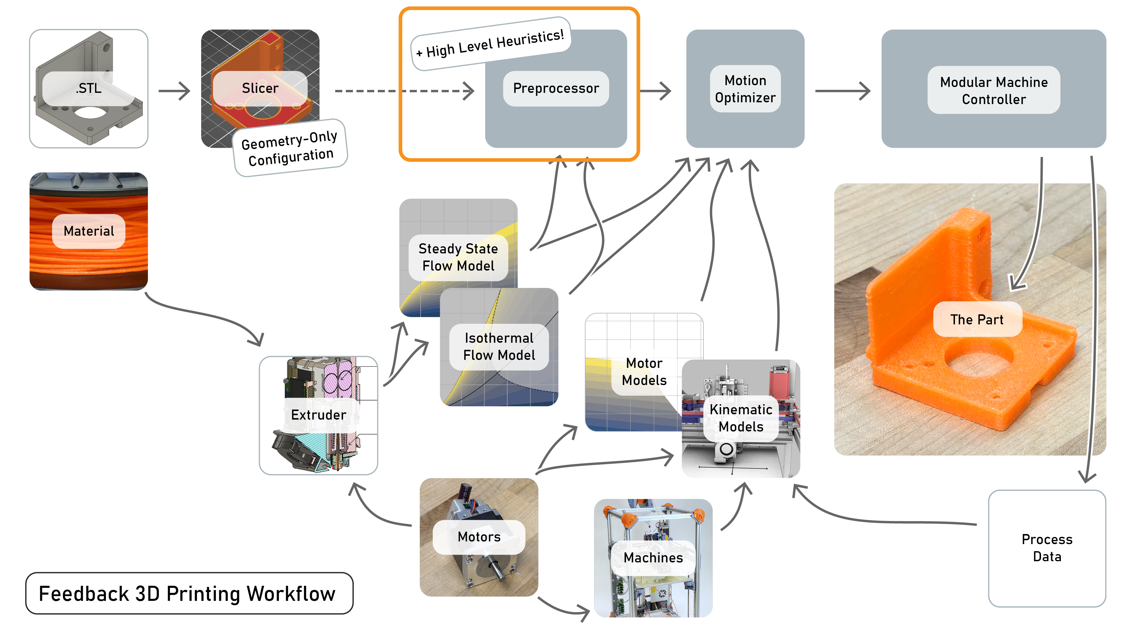
If we just optimize for speed, we would always print at the highest temperatures.
This can't be right - what are we missing?
The evolution of FFF Extruder Designs tells us... part cooling is important!
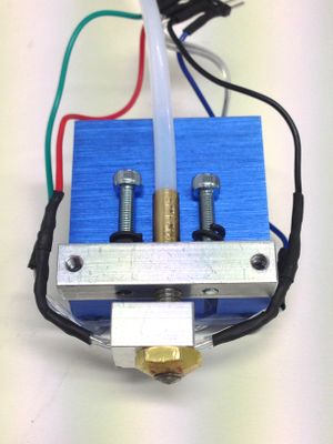
RepRap Mendel Hotend (no part cooling)
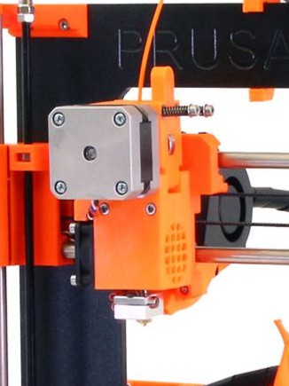
Prusa i3 MK1 (small part cooling fan)
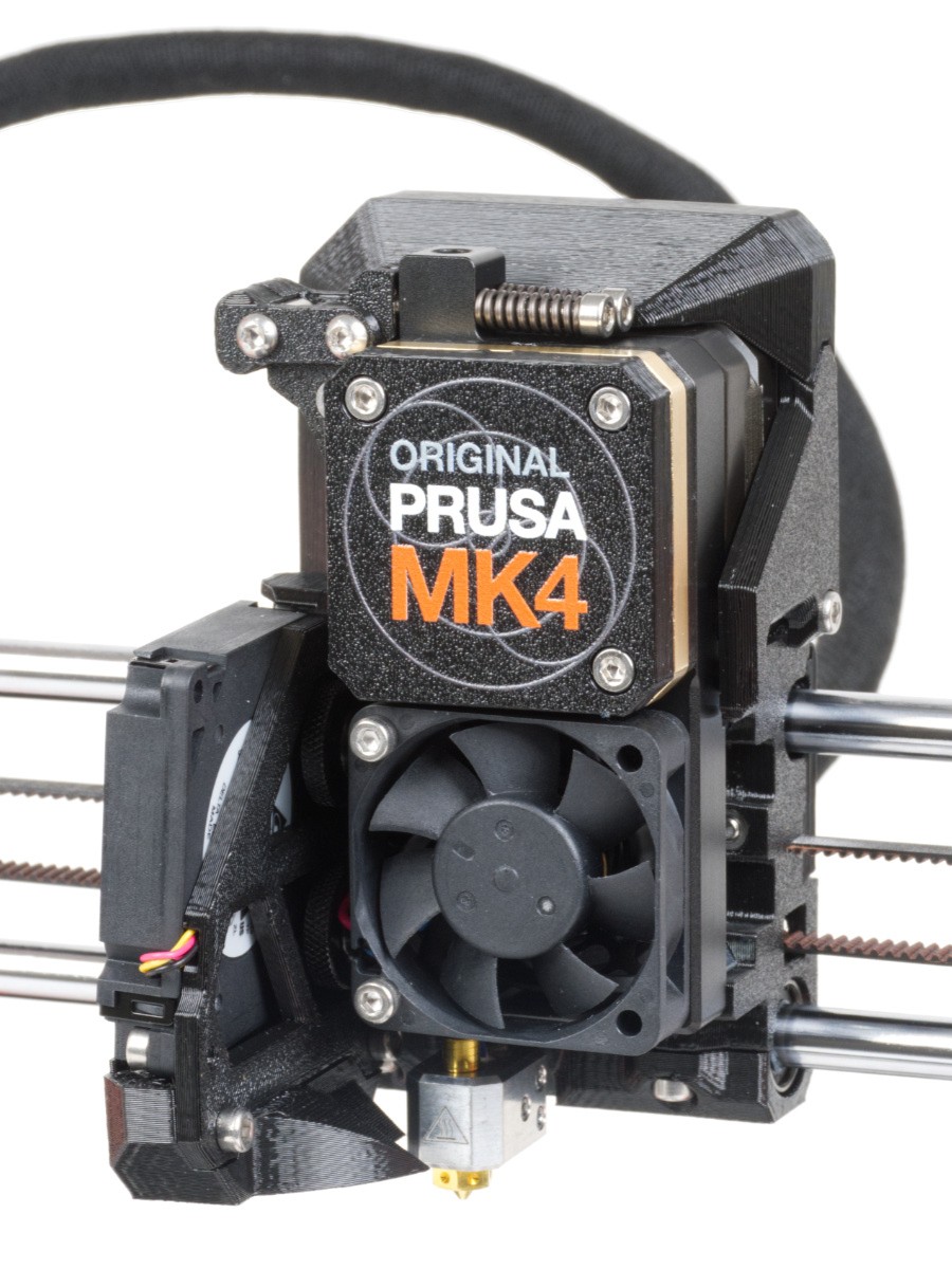
Prusa MK4 (bigger...)
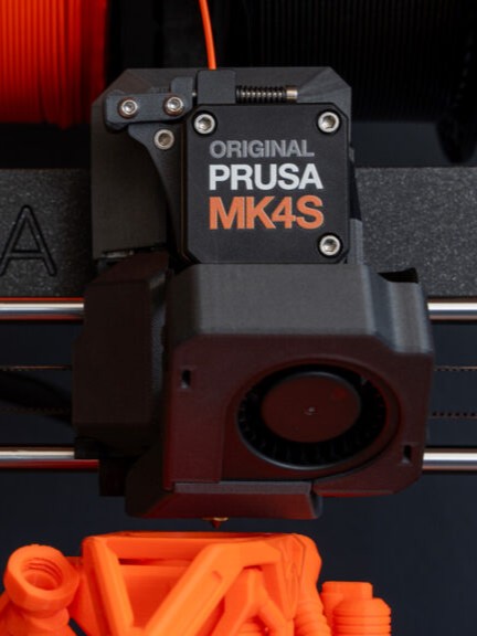
Prusa MK4S (bigger !)
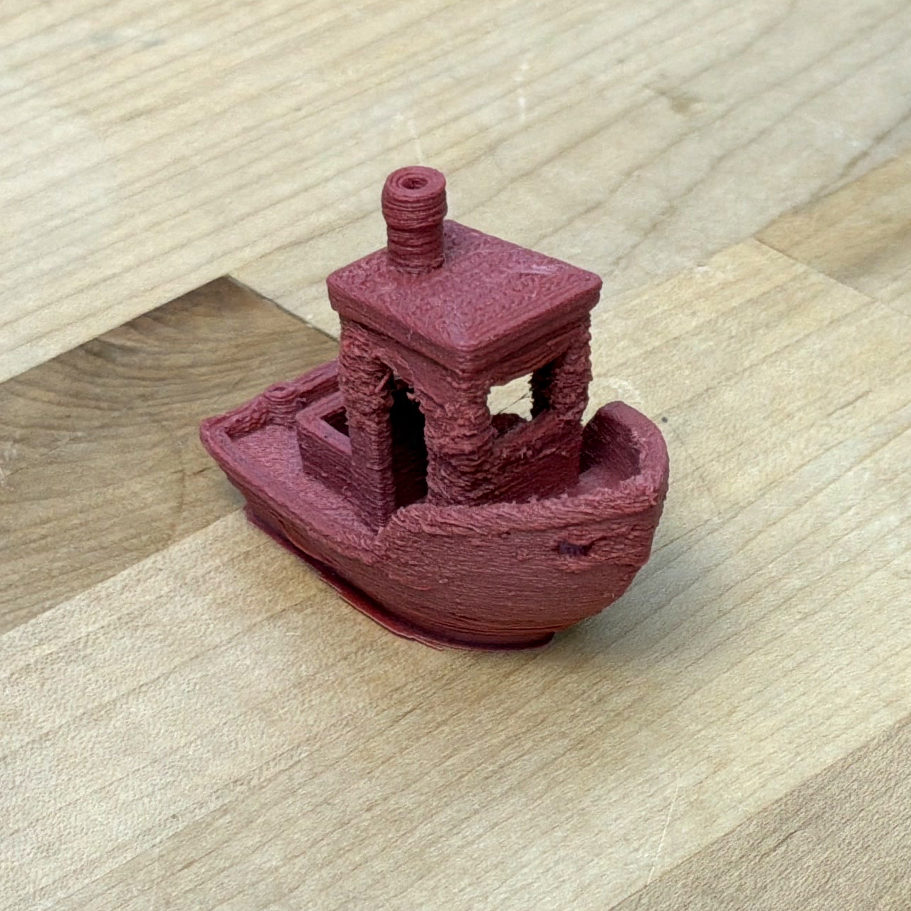
No cooling control.
With cooling control.
A Layer Cooling Model
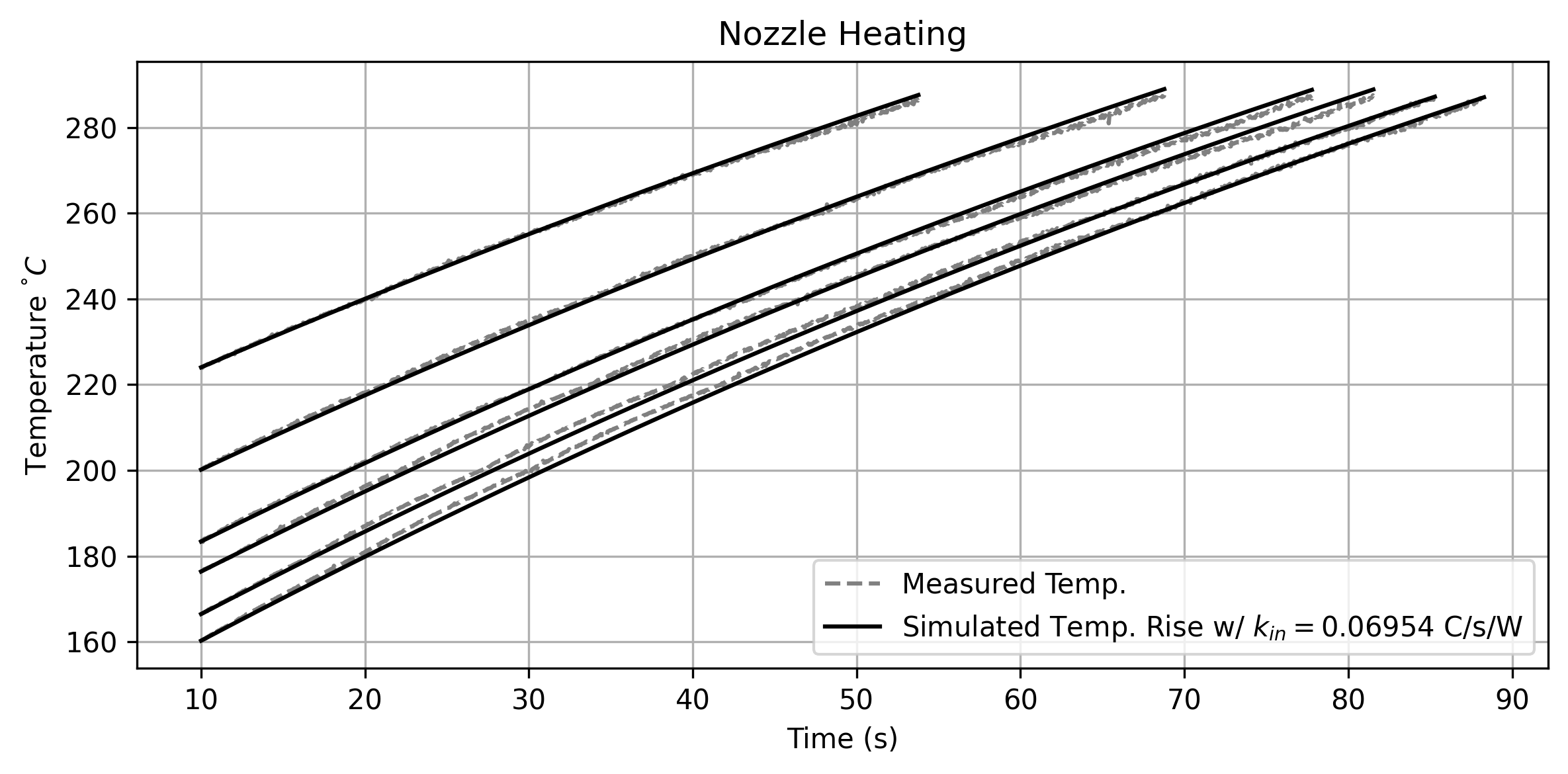
We know nozzle power input, giving us an energy basis for calorimetry.
We can measure energy loss to ambient vs. energy loss as a proportion of flowrate.
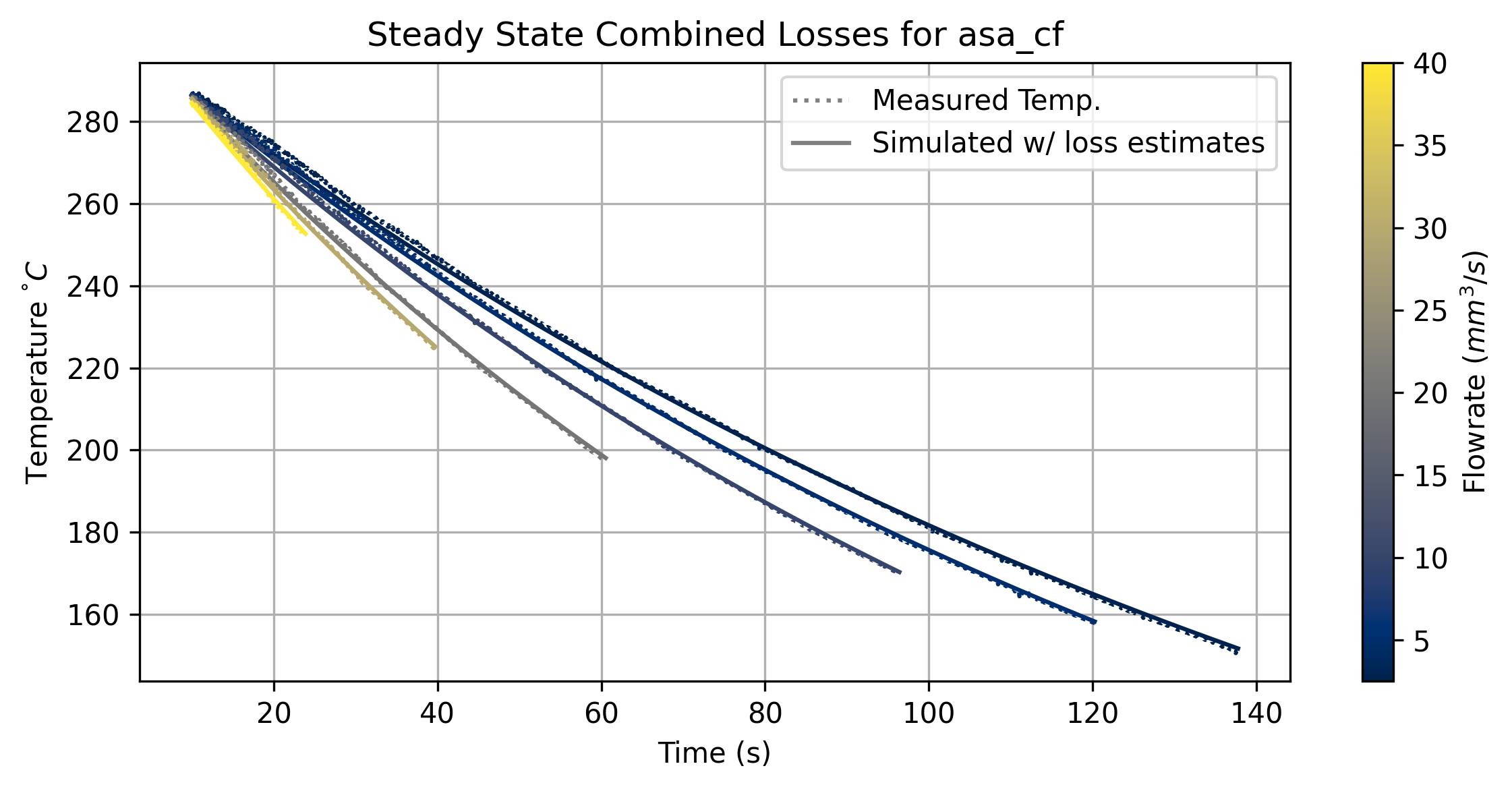
| Heater Temperature Loss |
| --- |
| $$ \frac{dT}{dt} = (T_{amb} - T) k_{loss} + {Q}(T_{amb} - T) k_{flow}$$ |
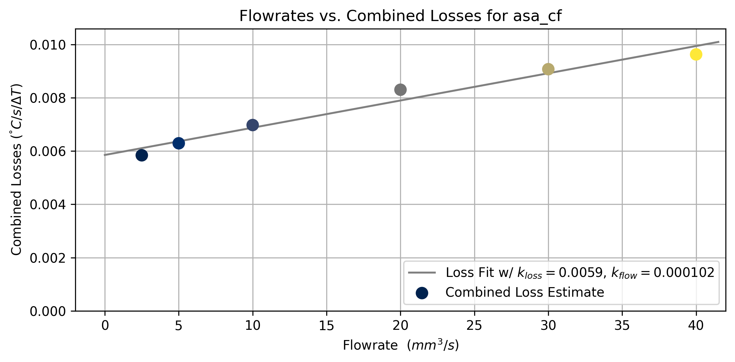
| Symbol | Value | Units | Source |
| --- | --- | ---: | --- |
| $T$ | Temperature of Flow | $^\\degree C$ | Measured |
| $T_{amb}$ | Ambient Temperature | $^\\degree C$ | Known |
| $Q$ | Volmetric Flowrate | $mm^3/s$ | Measured |
| $k_{loss}$ | Heat Loss to Ambient | $({C/s})/{\Delta T}$ | Model Fit |
| $k_{flow}$ | Heat Loss per unit of Flow | $({C/s \cdot (mm^3/s)})/{\Delta T}$ | Model Fit |
This lets us simulate required layer cooling times across nozzle temperatures.
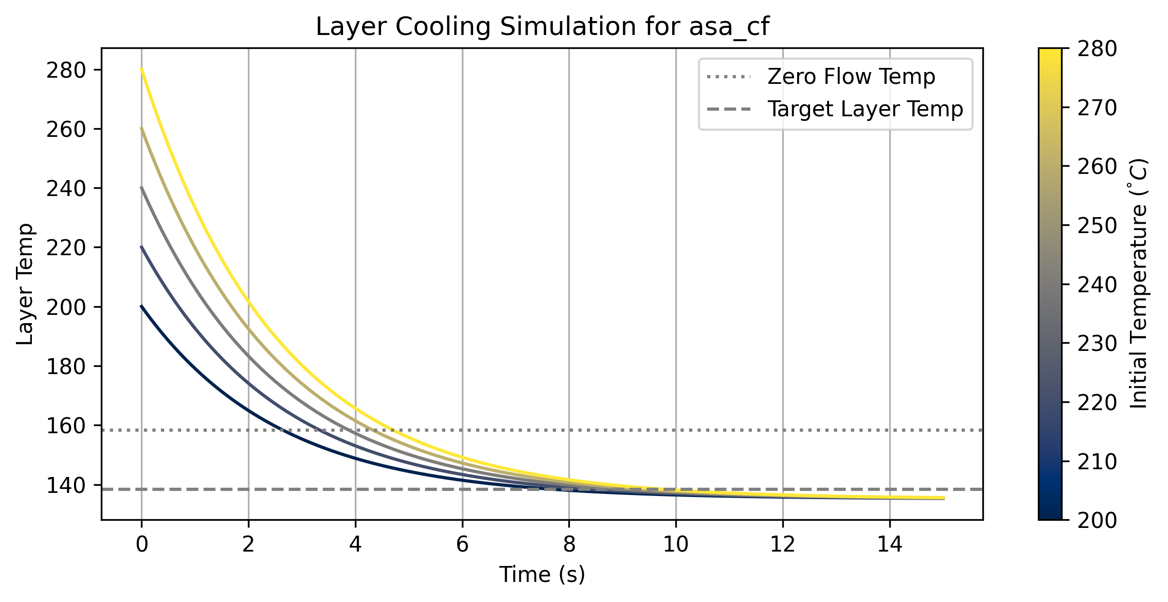
| Layer Cooling |
| --- |
| |
$$ t_{min} = -\tau \cdot log((T_{targ} - T_{eq})/(T_{noz} - T_{eq})) $$
$$ \tau = (C_{fil}) / (h_{air} + h_{layer}) $$
$$ T_{eq} = \frac{(h_{air} \cdot T_{amb} + h_{layer} \cdot T_{targ})}{(h_{air} + h_{layer})} $$
$$ h_{layer} = (\kappa_{fil} / H) \cdot l_{iface} $$
| Symbol | Value | Units | Source |
| :--- | :--- | ---: | --- |
| $H$ | Layer height | $mm$ | Part Geo. |
| $l_{iface}$ | Layer interface proportion | 0-1.0 | Part Geo. |
| $\kappa_{fil}$ | Filament conductivity | $W/m \cdot \Delta T$ | Estimated |
| $C_{fil}$ | Filament heat capacity | $J/m^2 \cdot \Delta T$ | Model Fit |
| $T_{noz}$ | Nozzle temperature | $\degree C$ | Direct Measurement |
| $T_{targ}$ | Cooling target temperature | $\degree C$ | From Flow Models |
| $T_{ambient}$ | Chamber air temperature | $\degree C$ | Known |
| $h_{air}$ | Heat transfer to air | $W/m^2 \cdot \Delta T$ | Estimated |
| $h_{layer}$ | Heat transfer to layer below | $W/m^2 \cdot \Delta T$ | Via $fil_k$ |
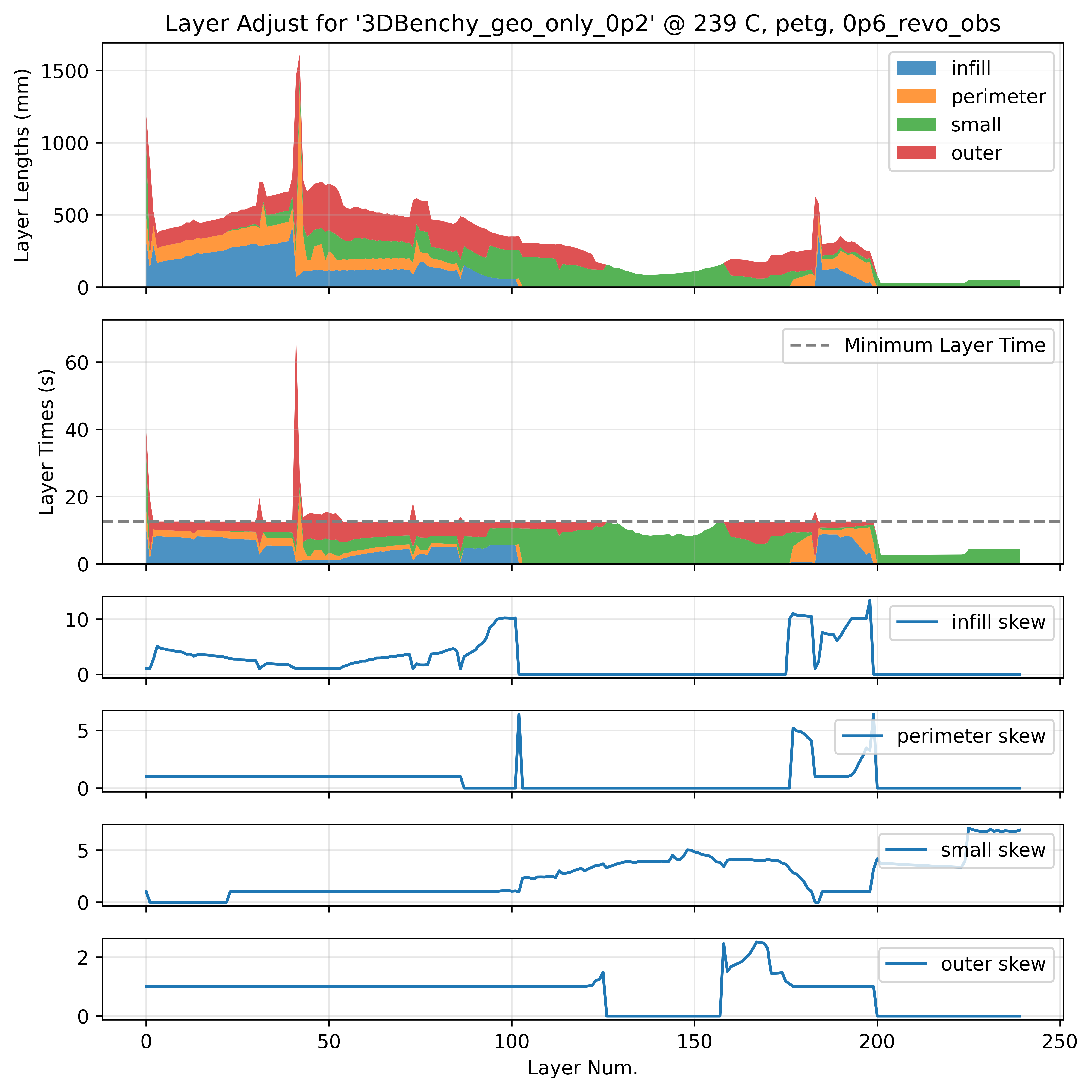
Planned rates can be skewed to hit target minimum layer times.
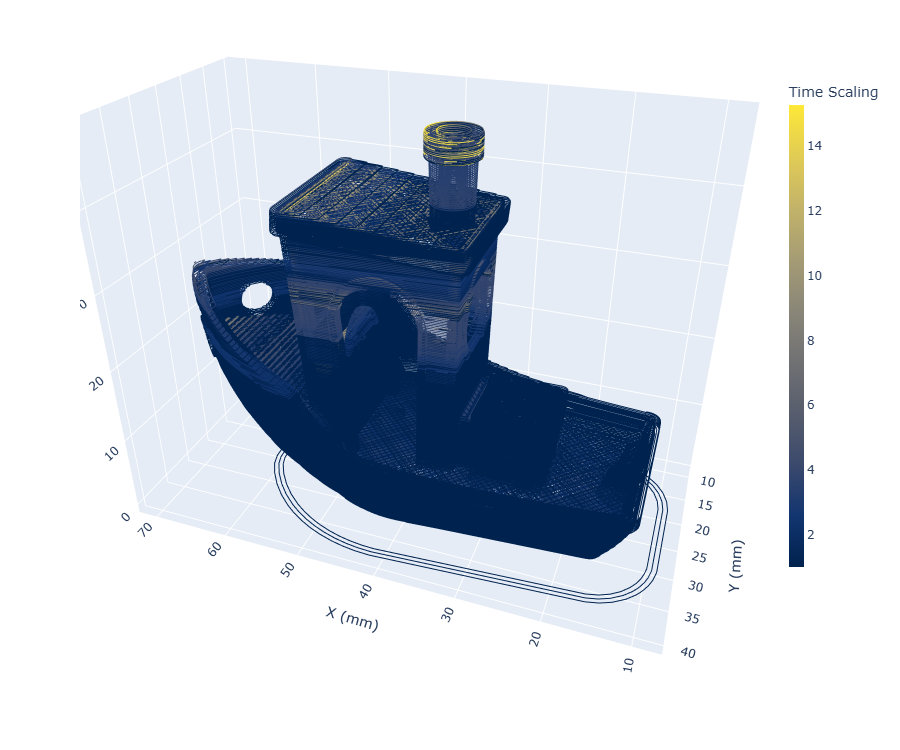
Above: FFF path plan with rates-scaling applied to enforce the minimum layer time
set by the layer cooling simulation.
Hot: slow (more skew), cold: as-planned.
Hot: slow (more skew), cold: as-planned.
We prioritize slowing hidden features, to minimize changes in appearance.
* This scaling step exists in the state-of-the-art. Estimates for filament heat capacity
from nozzle data and the layer cooling simulation formulation are my own.
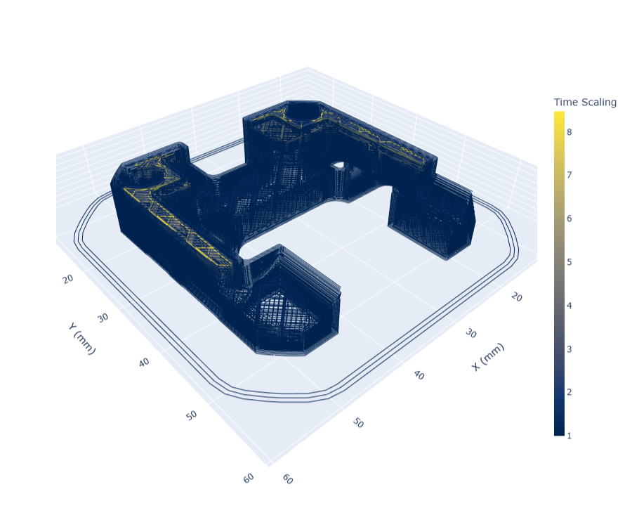
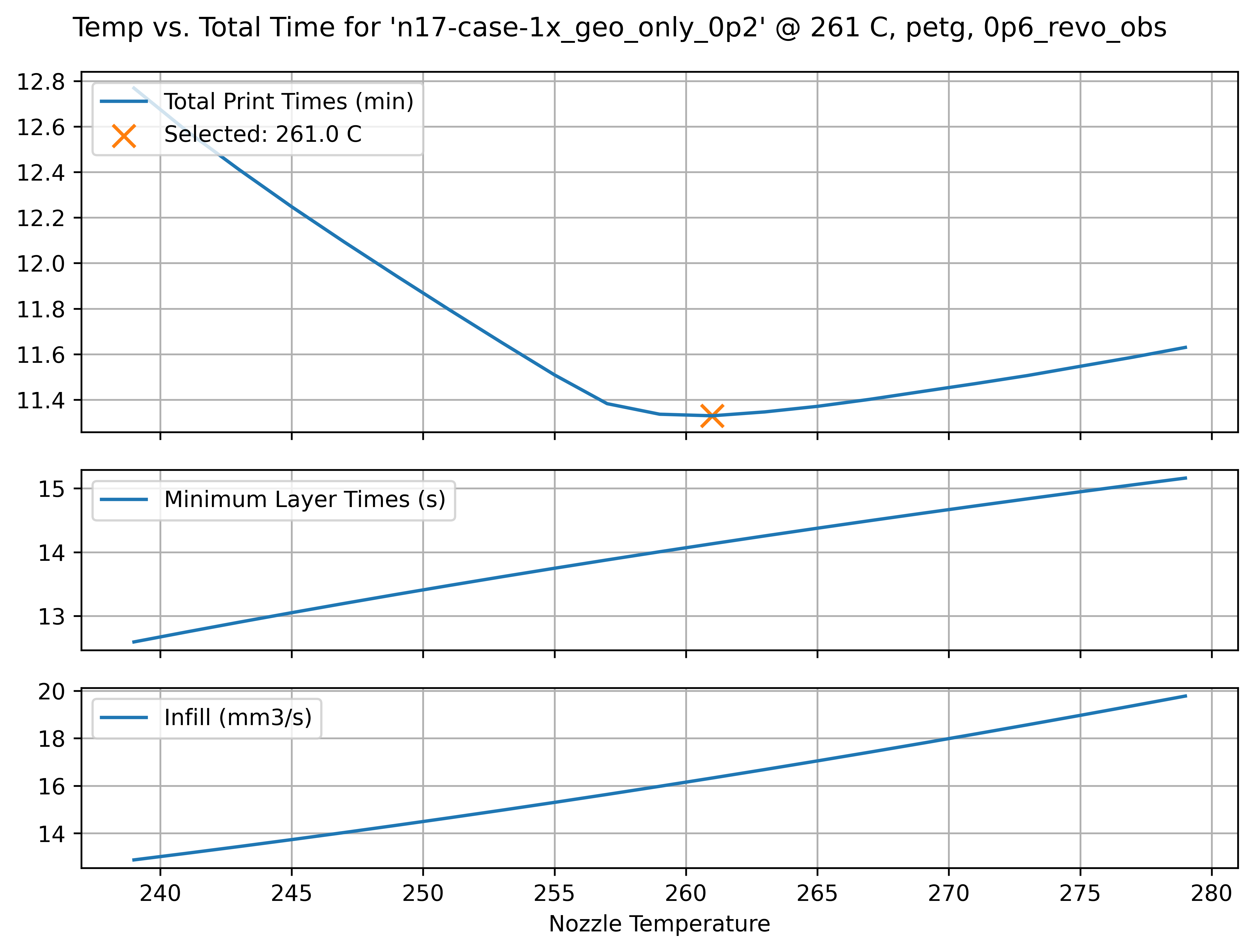
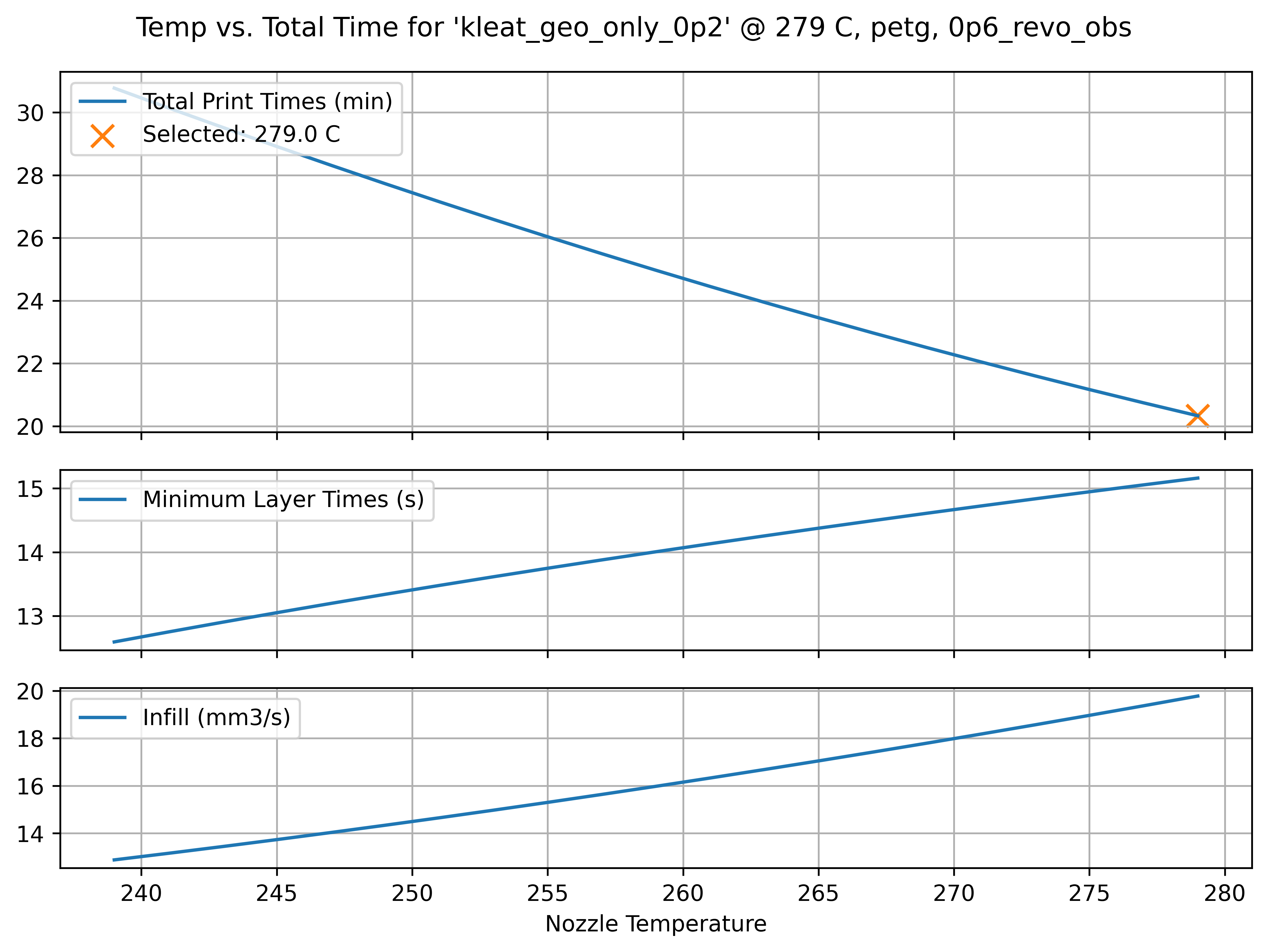
We can see that small parts tend towards $T_{min}$, but temperature selection quickly increases.
~65x80mm part @ 239 C
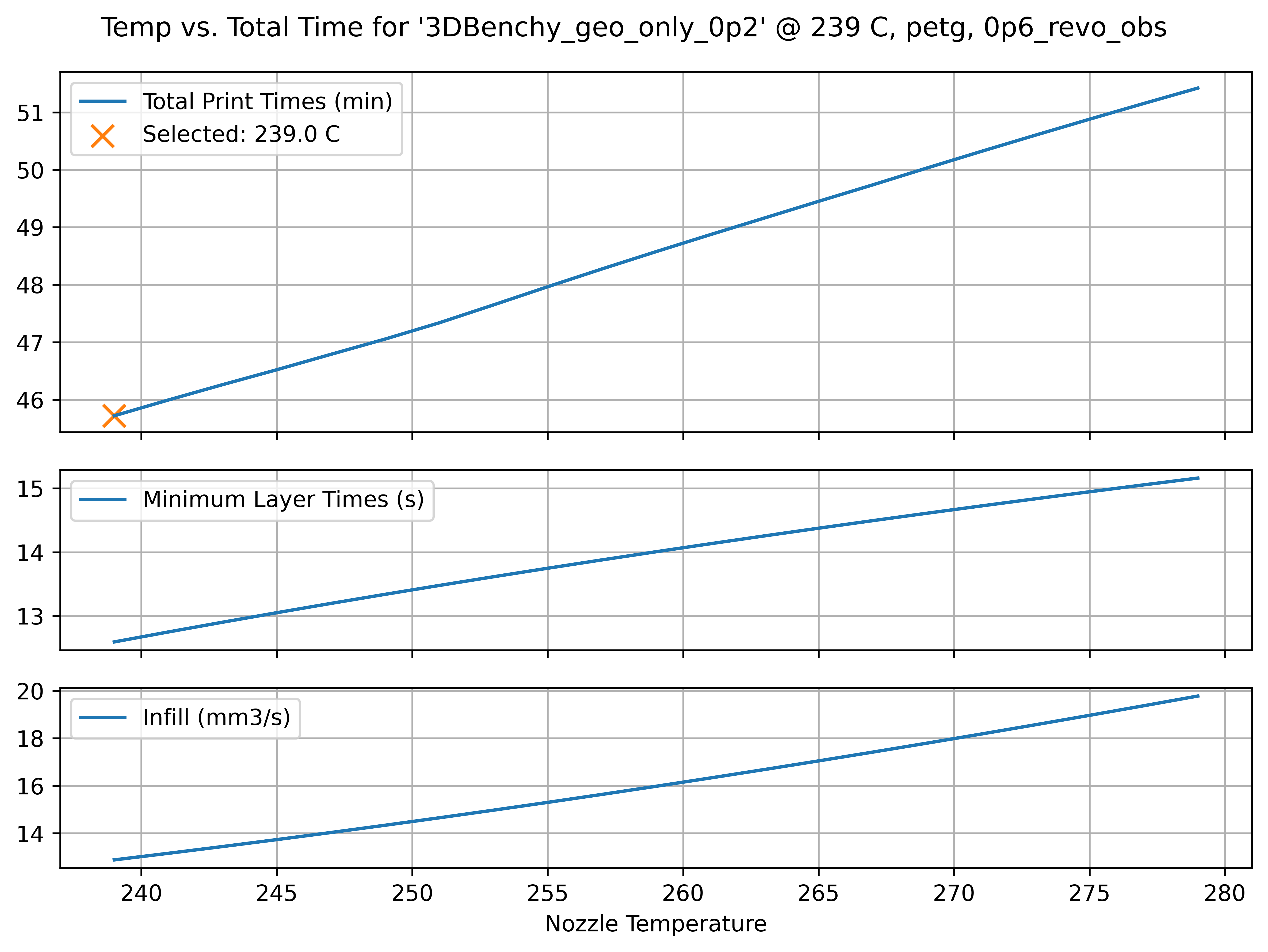
~80x80mm @ 261 C (11% Speedup)
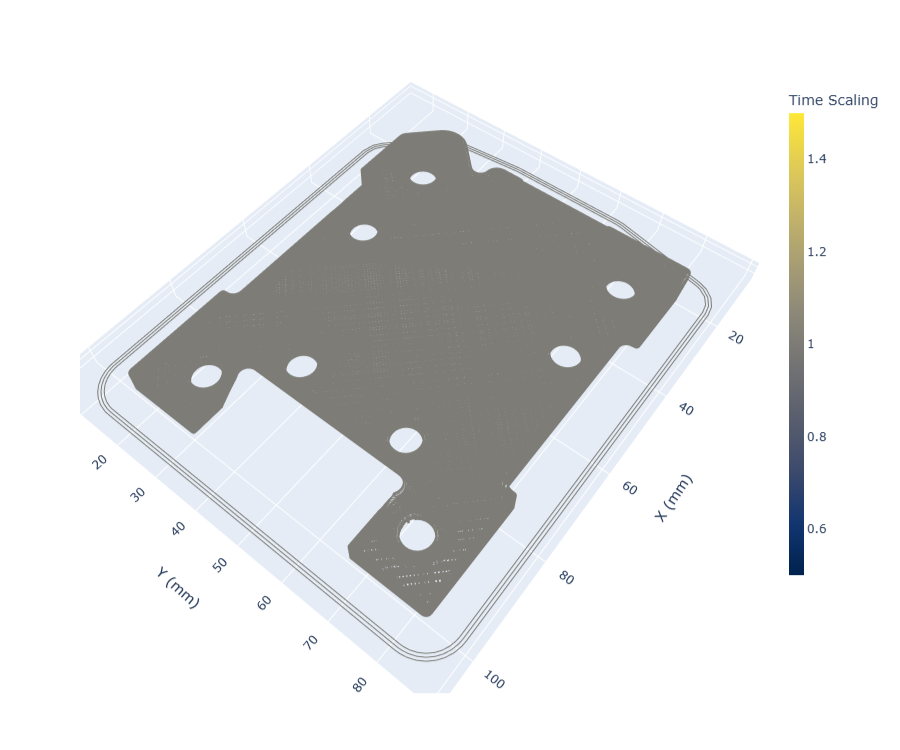
~80x130mm @ 279 C (50% Speedup)
But we still need to actually run the printer.
Can we include process and motion dynamics in one optimization?
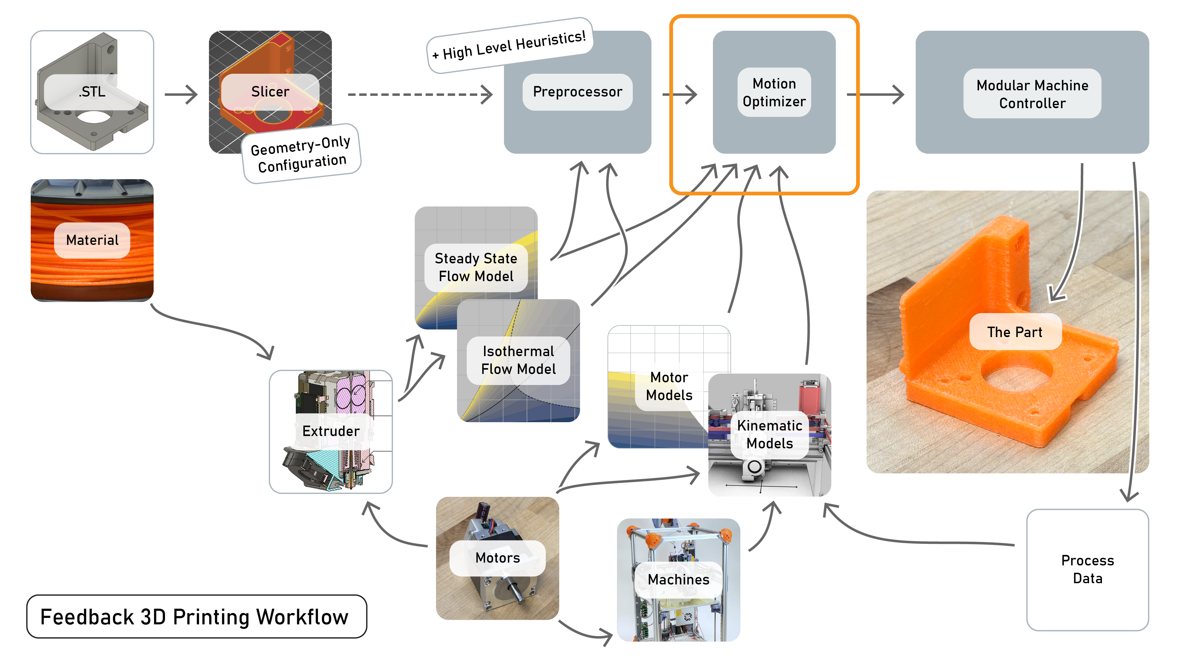
Because the solver is developed using a general purpose optimization framework,
we can extend it with some flexibility.
We add to the trajectory...
$$
\overset{q_{trg}(s)}{\begin{bmatrix} 0 \\ \vdots \\ \vdots \\ \vdots \\ n \end{bmatrix}}
\
\overset{v_{max}(s)}{\begin{bmatrix} 0 \\ \vdots \\ \vdots \\ \vdots \\ n \end{bmatrix}}
\
\overset{I_{prop,e}(s)}{\begin{bmatrix} 0 \\ \vdots \\ \vdots \\ \vdots \\ n \end{bmatrix}}
\
\overset{\dot{I}_{prop,e}(s)}{\begin{bmatrix} 0 \\ \vdots \\ \vdots \\ \vdots \\ n \end{bmatrix}}
$$
Extrusion related values:
$q_{trg}$ extrusion widths: $mm^3/mm$
$v_{max}$ rate limits encode cooling, flow heuristics
$I_{prop,e}$ extruder $I$ deployment
$\dot{I}_{prop,e}$ extruder $I$ slewrate
$q_{trg}$ extrusion widths: $mm^3/mm$
$v_{max}$ rate limits encode cooling, flow heuristics
$I_{prop,e}$ extruder $I$ deployment
$\dot{I}_{prop,e}$ extruder $I$ slewrate
Solver selects:
$$
\overset{v(s)}{\begin{bmatrix} 0 \\ \vdots \\ \vdots \\ \vdots \\ n \end{bmatrix}}
$$
Velocities at each point, $v(s)$
same as before!
same as before!
We calculate ...
$$
\overset{q_{out}(s)}{\begin{bmatrix} 0 \\ \vdots \\ \vdots \\ \vdots \\ n \end{bmatrix}}
\
\overset{T_{melt}(s)}{\begin{bmatrix} 0 \\ \vdots \\ \vdots \\ \vdots \\ n \end{bmatrix}}
\
\overset{F(s)}{\begin{bmatrix} 0 \\ \vdots \\ \vdots \\ \vdots \\ n \end{bmatrix}}
\
\overset{\Delta F(s)}{\begin{bmatrix} 0 \\ \vdots \\ \vdots \\ \vdots \\ n \end{bmatrix}}
\
\overset{q_{in}(s)}{\begin{bmatrix} 0 \\ \vdots \\ \vdots \\ \vdots \\ n \end{bmatrix}}
$$
$q_{out}$ is set directly.
$T_{melt}$* uses an energy model and both flow models to estimate real melt flow temperature.
Extrusion Force $F$ uses the isothermal flow model, at $T_{melt}$
The required flow in to the melt zone $q_{in}$ is calculated using $\Delta F$ and the compressibility of the filament at $T_{melt}$
$T_{melt}$* uses an energy model and both flow models to estimate real melt flow temperature.
Extrusion Force $F$ uses the isothermal flow model, at $T_{melt}$
The required flow in to the melt zone $q_{in}$ is calculated using $\Delta F$ and the compressibility of the filament at $T_{melt}$
Extruder actuator...
$$
\overset{I_{req,e}(s)}{\begin{bmatrix} 0 \\ \vdots \\ \vdots \\ \vdots \\ n \end{bmatrix}}
\
\overset{I_{lim,e}(s)}{\begin{bmatrix} 0 \\ \vdots \\ \vdots \\ \vdots \\ n \end{bmatrix}}
\
\overset{\dot{I}_{req,e}(s)}{\begin{bmatrix} 0 \\ \vdots \\ \vdots \\ \vdots \\ n \end{bmatrix}}
\
\overset{\dot{I}_{lim,e}(s)}{\begin{bmatrix} 0 \\ \vdots \\ \vdots \\ \vdots \\ n \end{bmatrix}}
$$
Adding the required and available extruder motor currents and current slew rates.
This step uses the actuator model.
Again, real limits are scaled by $I_{prop}, \dot{I}_{prop}$, heuristics!
Again, real limits are scaled by $I_{prop}, \dot{I}_{prop}$, heuristics!
Add to the cost two heuristics for extruder inflow.*
$$
\begin{aligned}
\text{cost}&+=\sum_{s} \Bigl[\, q_{in,2big}(s) \Bigr] + \Bigl[\, \dot{q}_{in,2big}(s) \Bigr] \\
\end{aligned} \\
\min_{v(s)} \; \text{cost}
$$
As before, minimize the cost function by optimizing over $v(s)$.
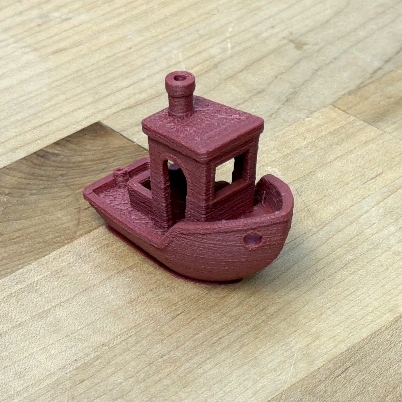
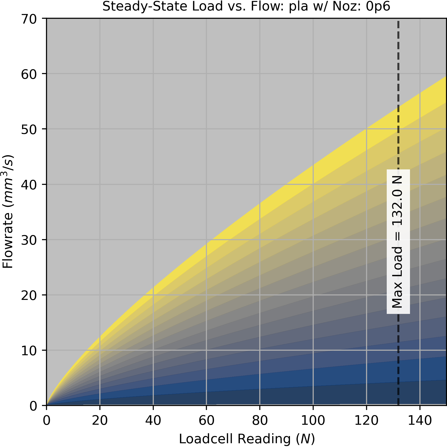
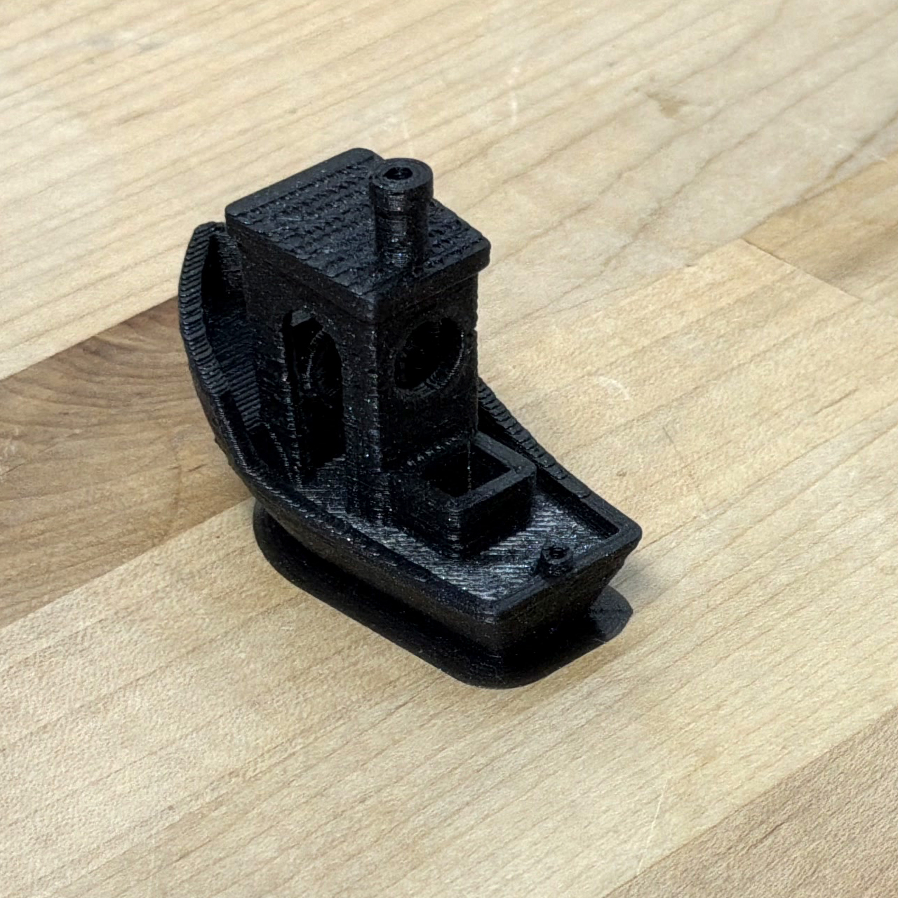
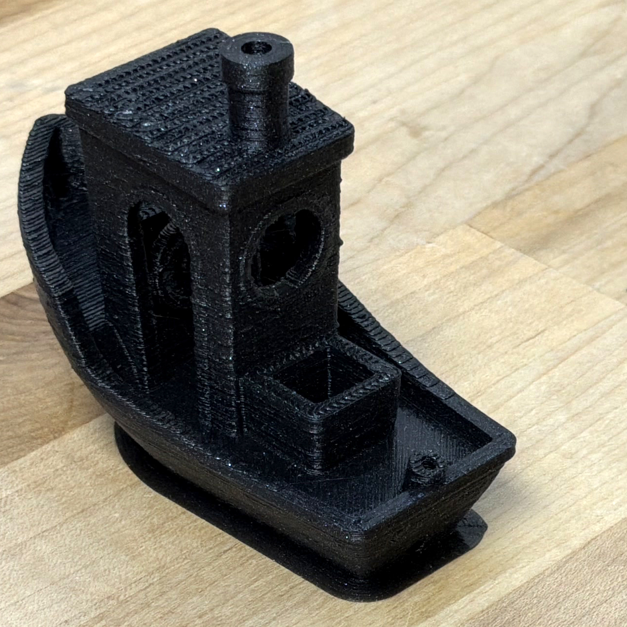
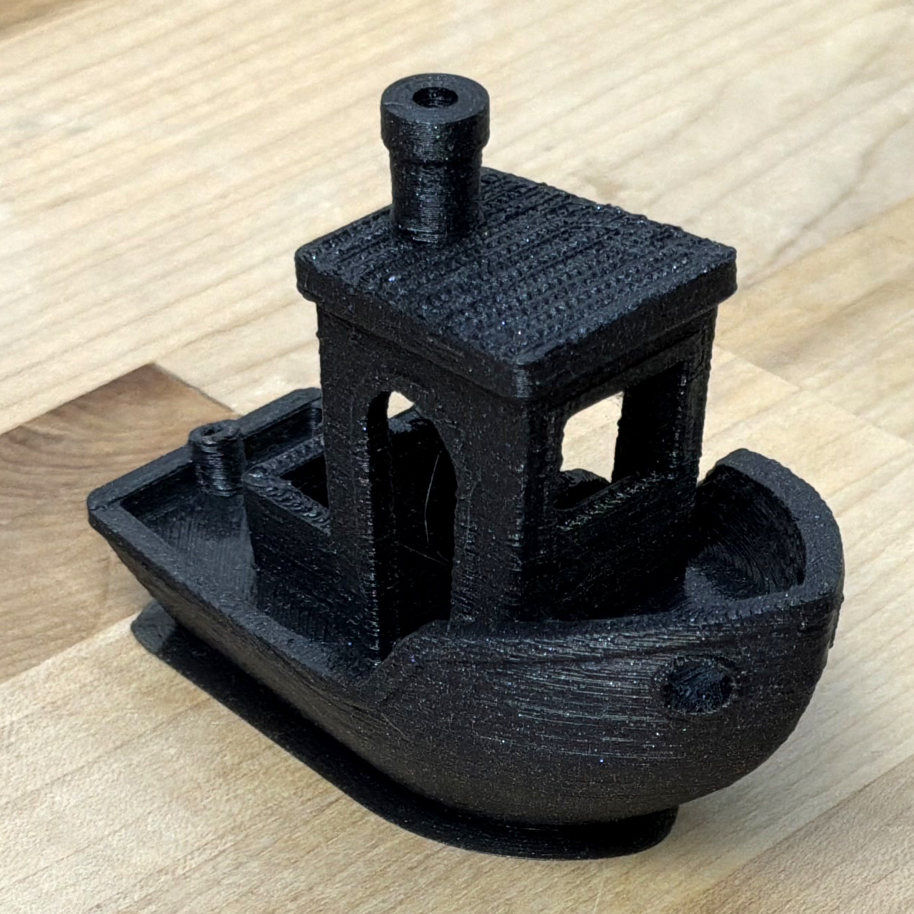
PLA, 0.6mm Brass Nozzle, Benchy, Big Benchy (1.5x)
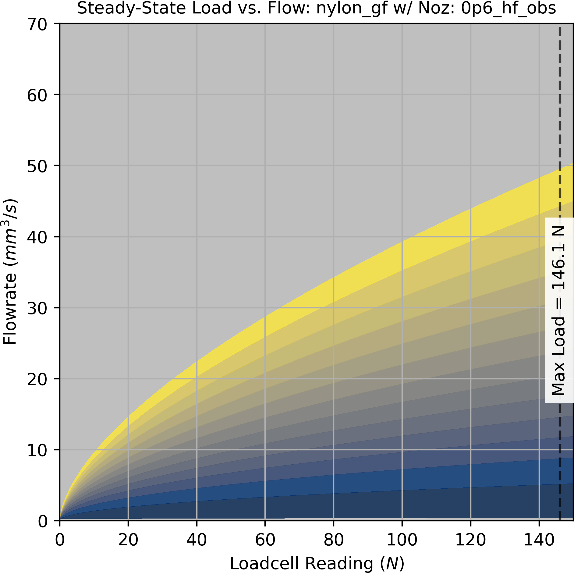
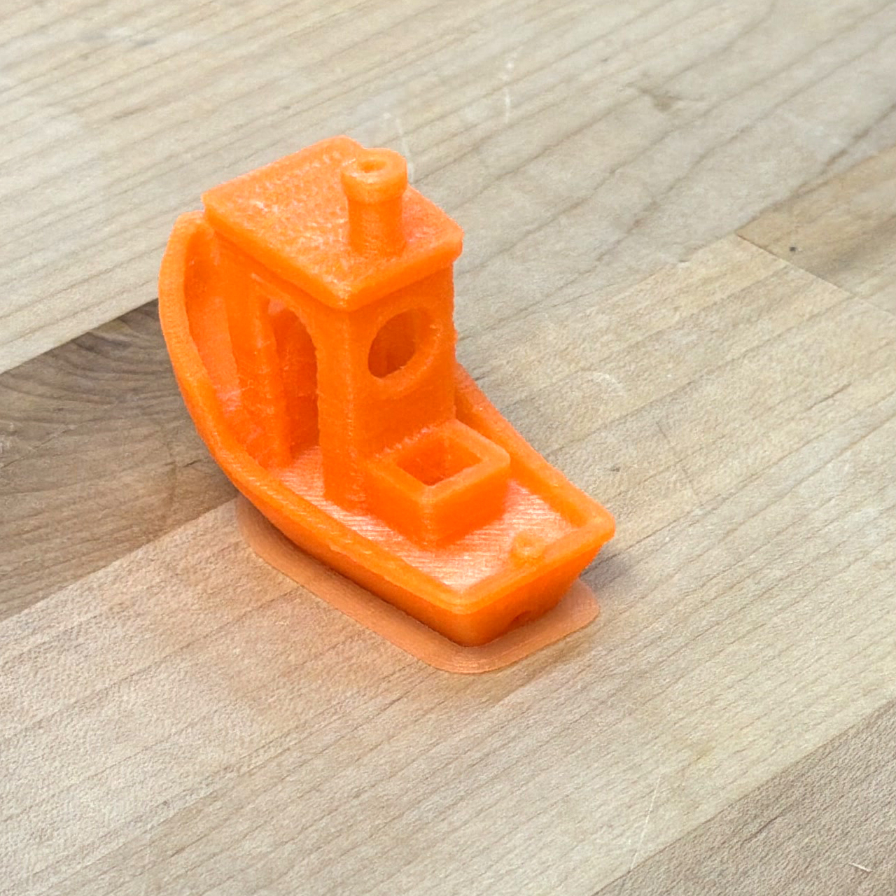
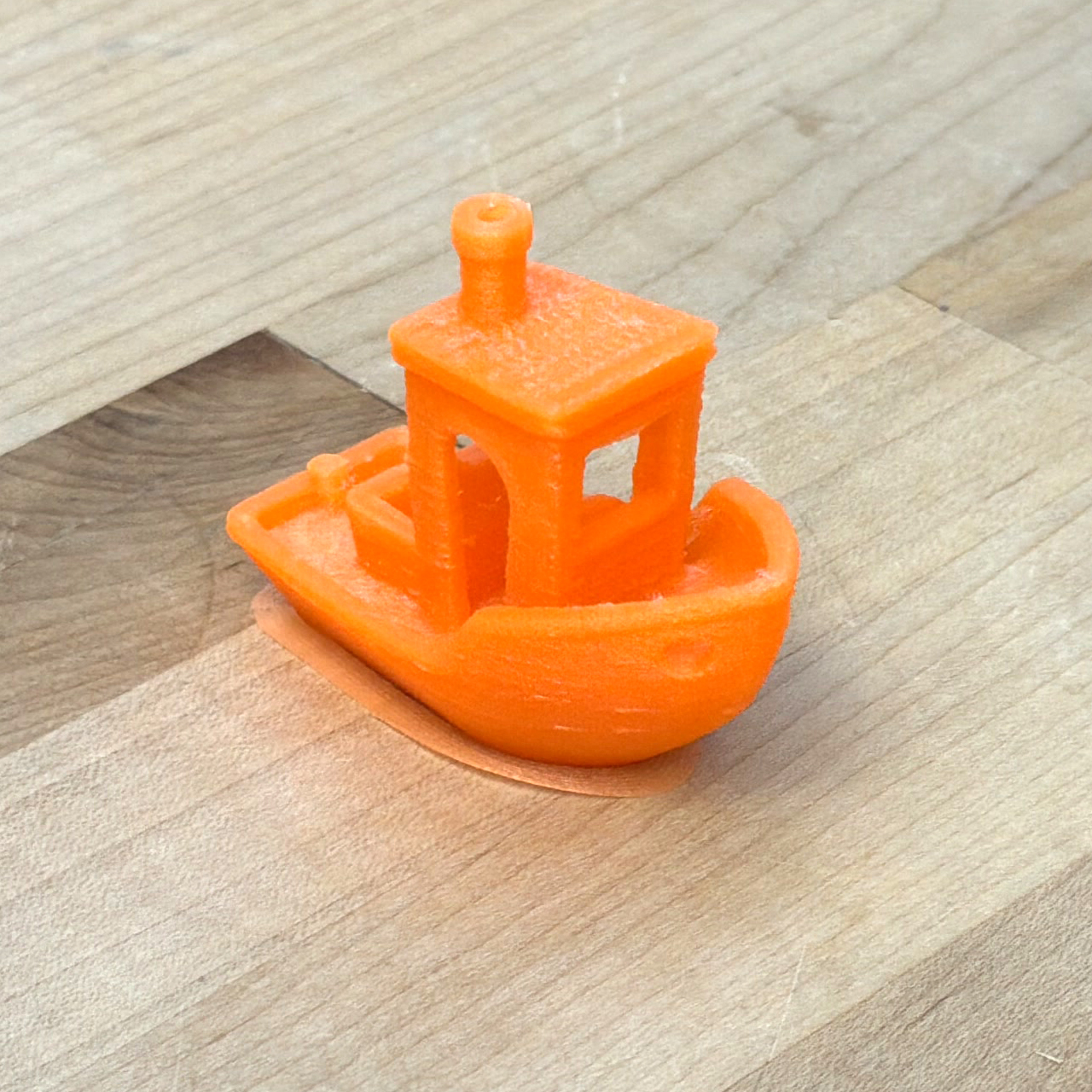
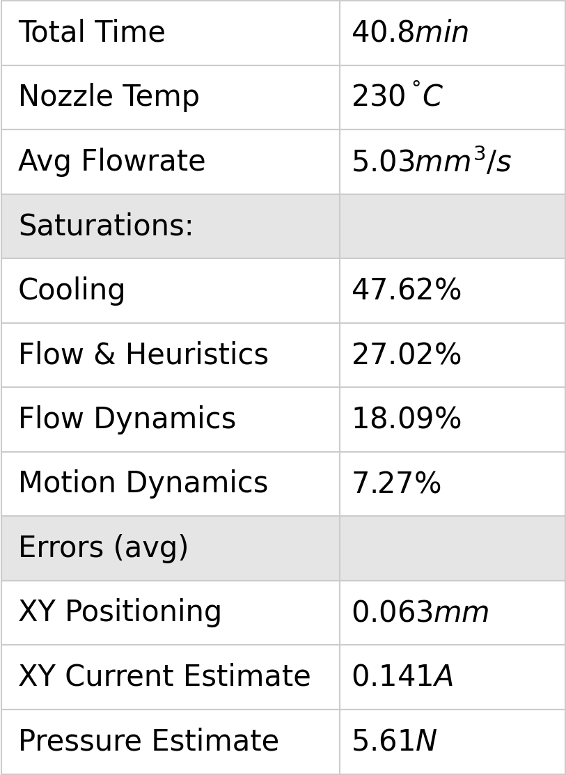
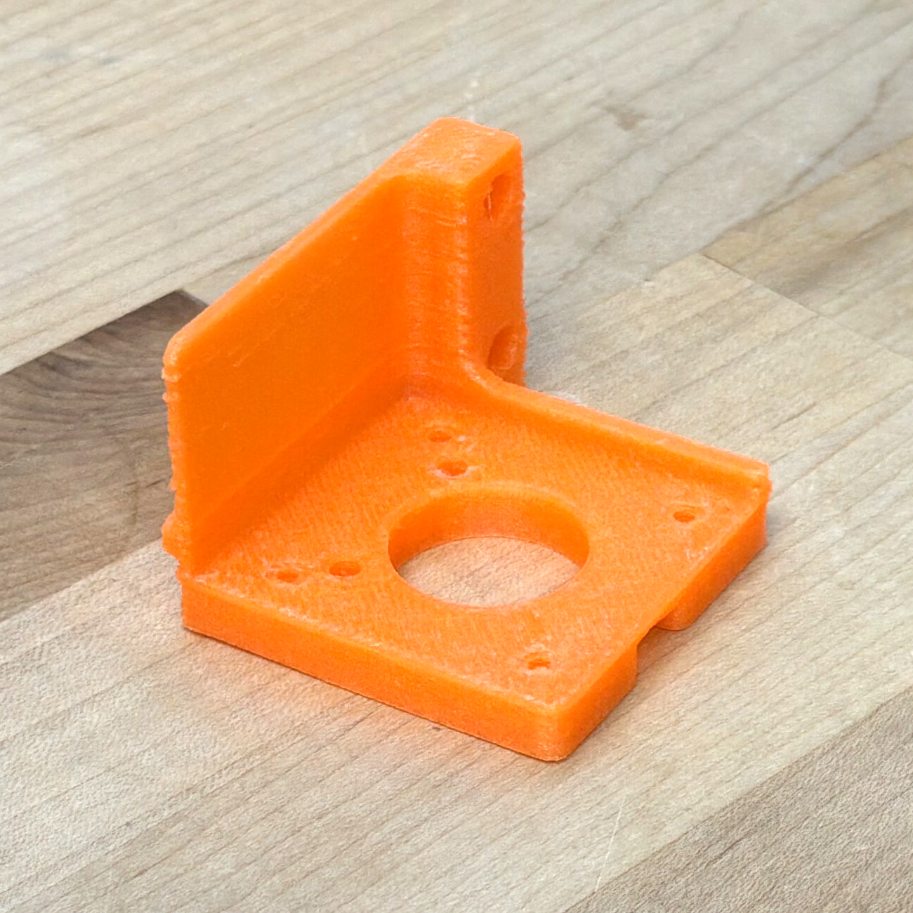
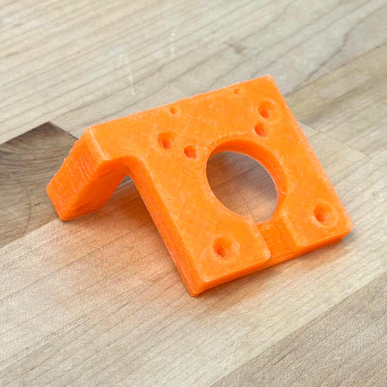
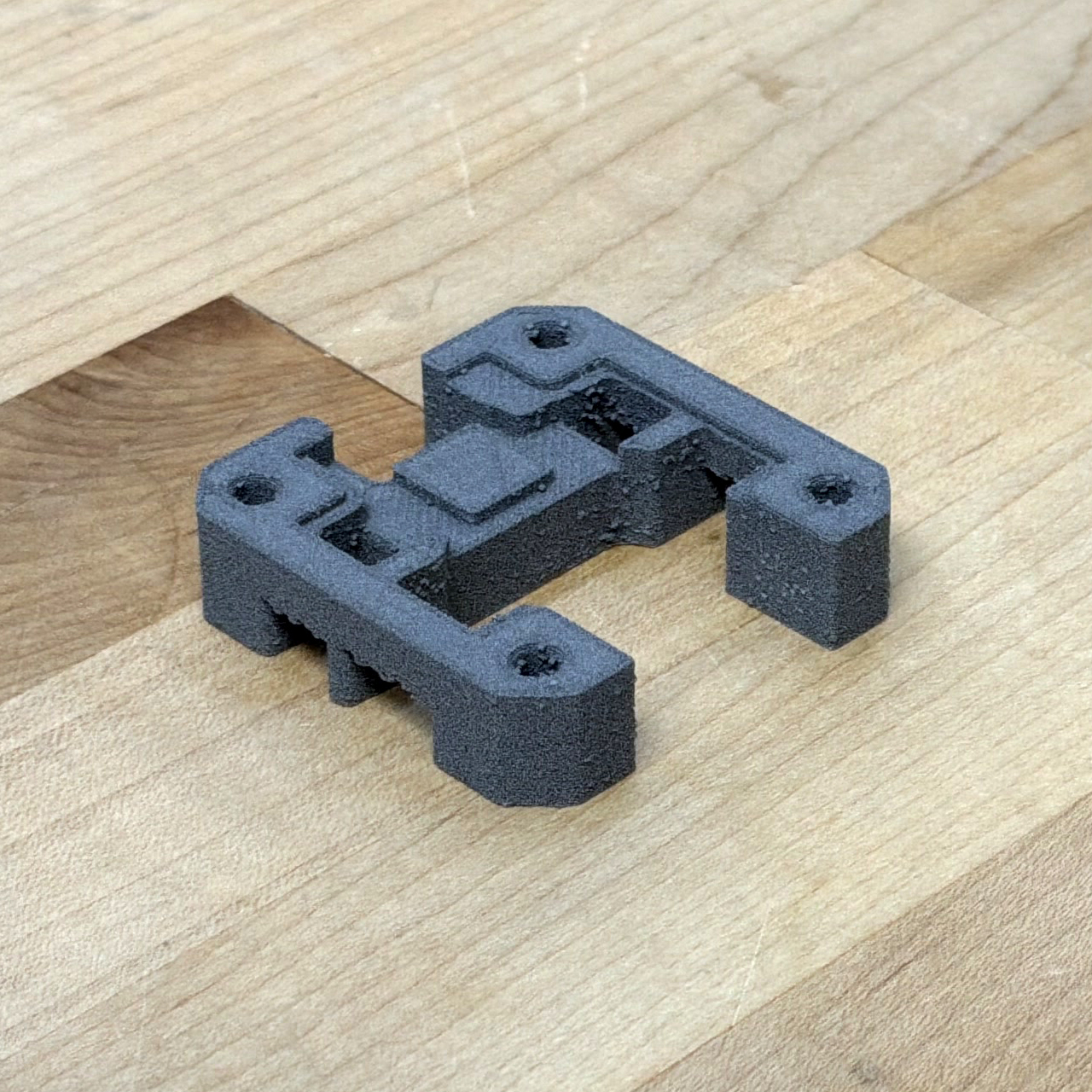
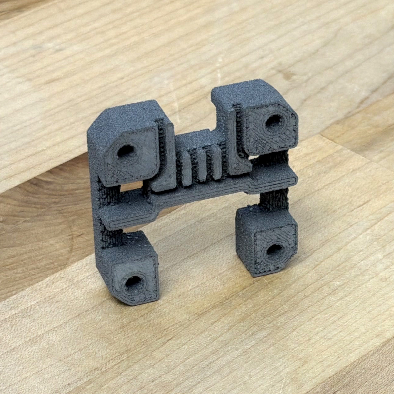
Nylon, Glass Fill, 0.6mm High Flow Coated Nozzle, Benchy, Motor Mount.
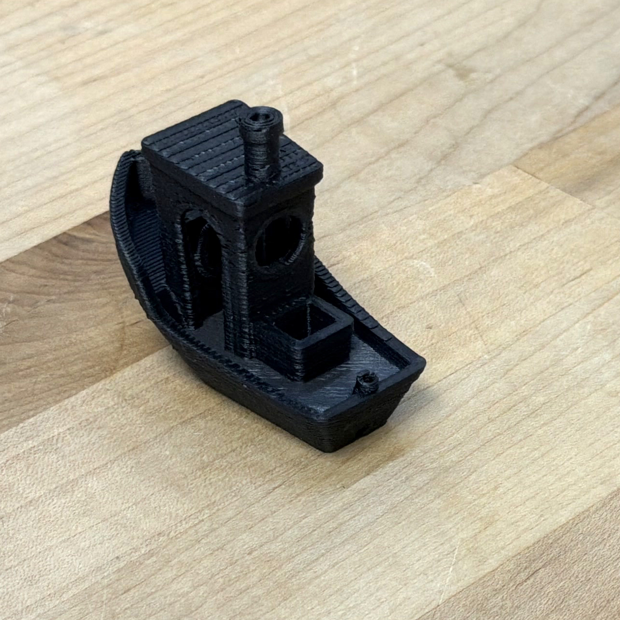
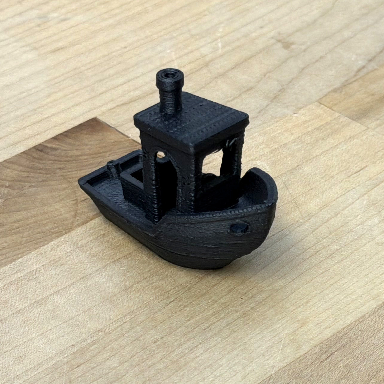
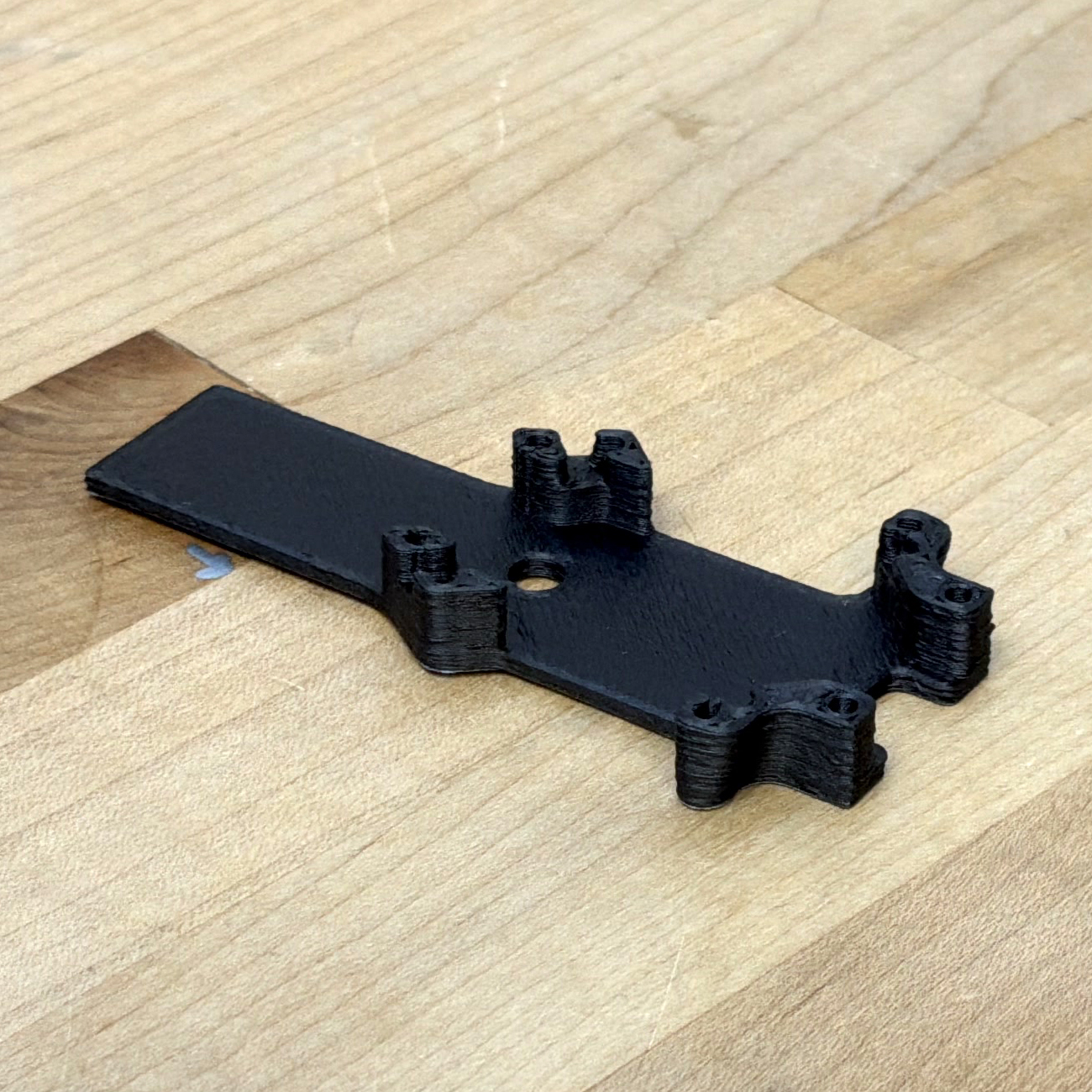
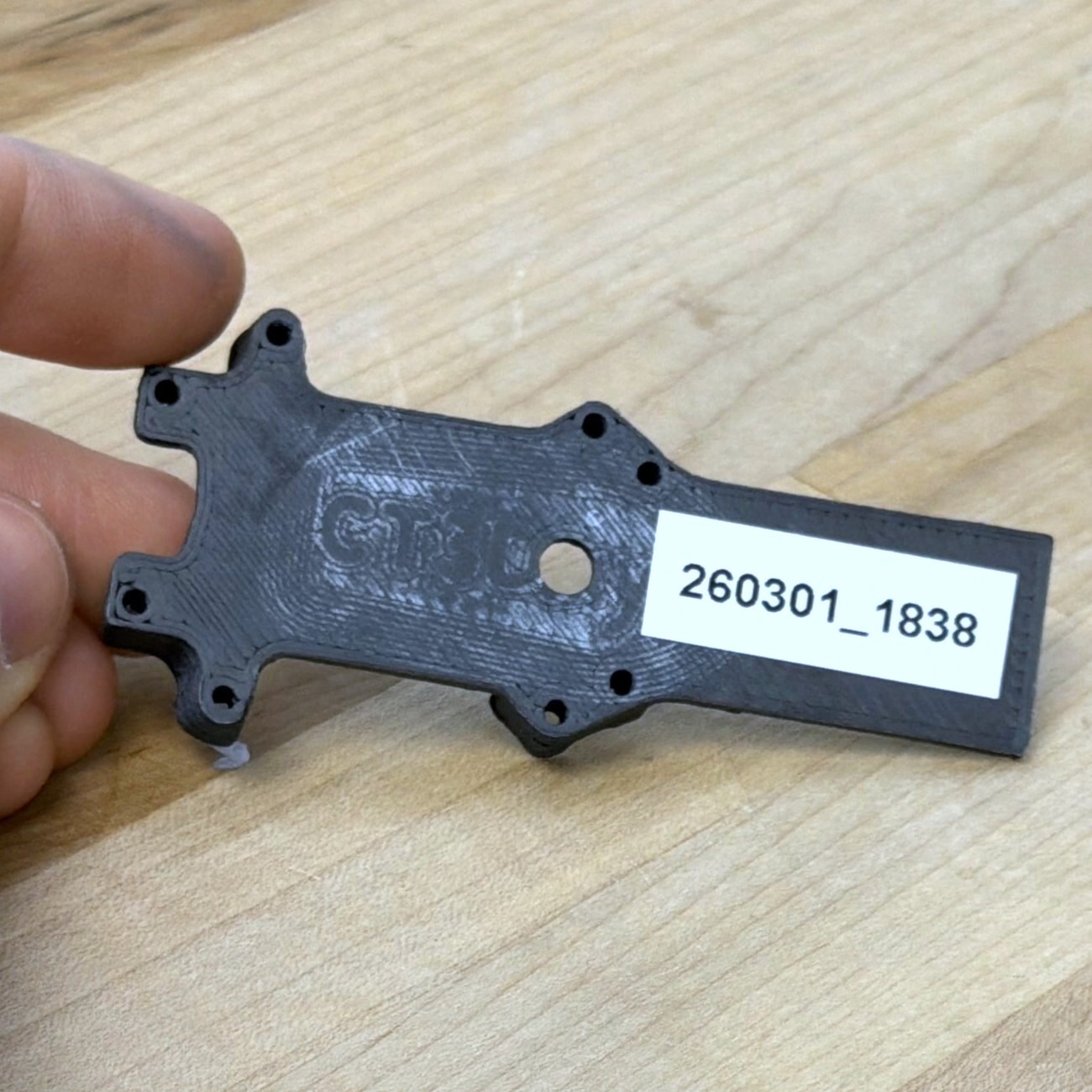
PCBlend, Carbon Fill, 0.6mm High Flow Coated Nozzle, Benchy, Drone Part.
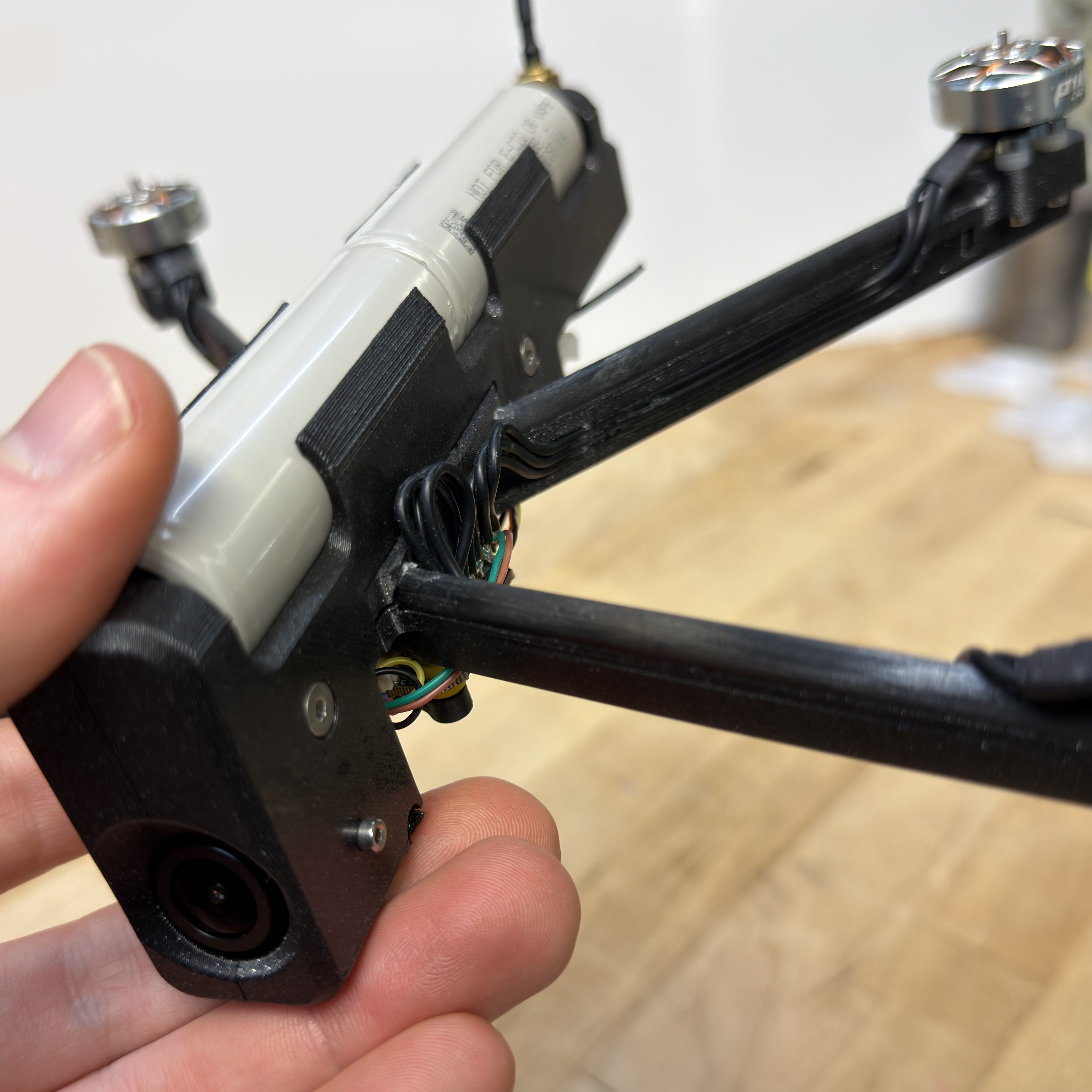
Manually glue-ing in carbon tubes...
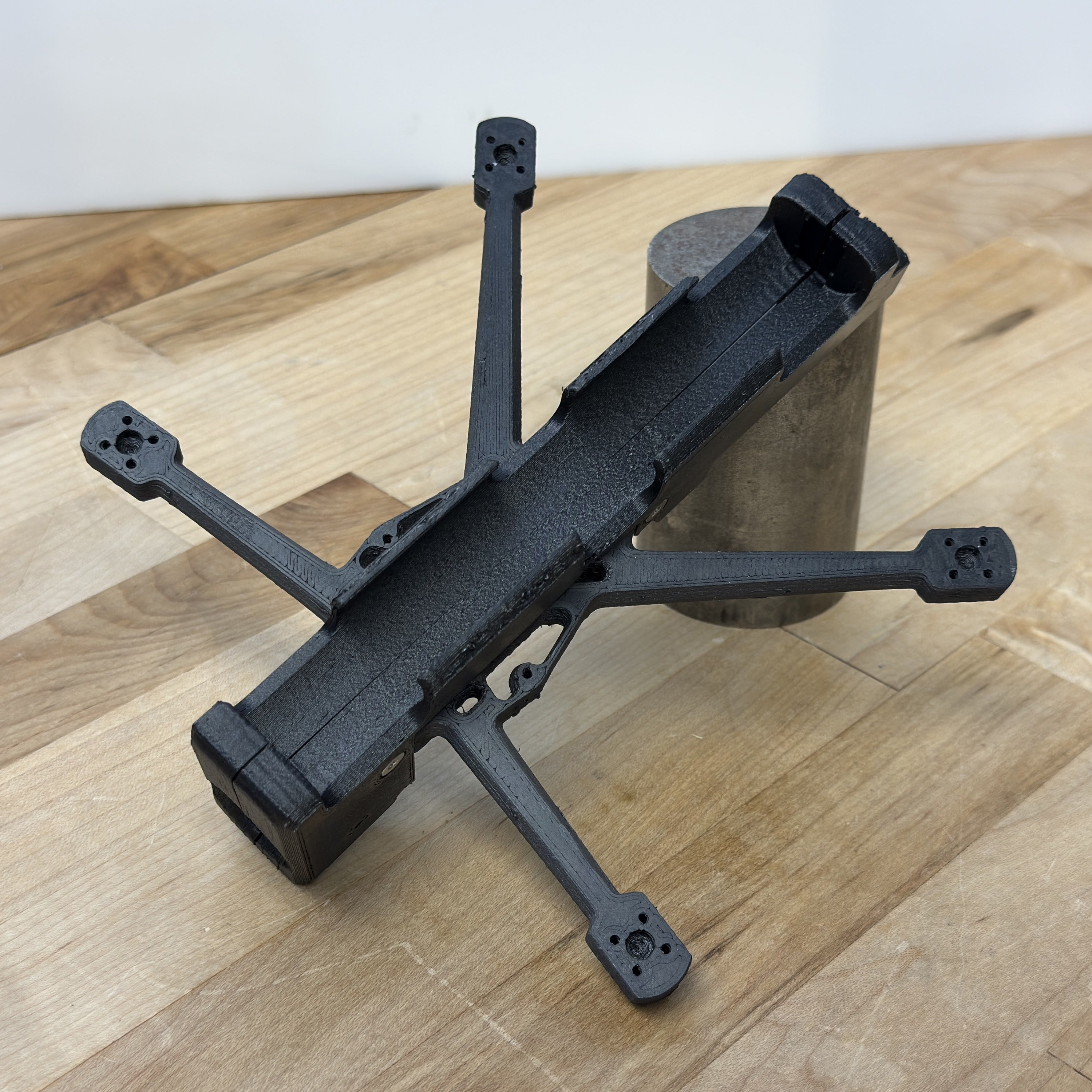
vs. Carbon Filament !
Timberfill, 0.4mm High Flow Coated Nozzle,* Benchy, Moai (Yassified).
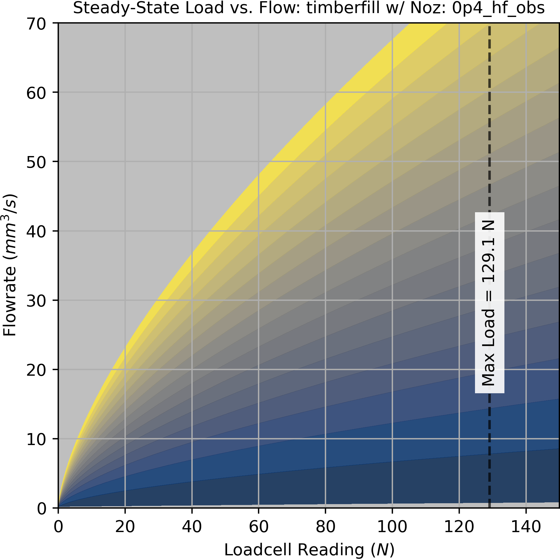
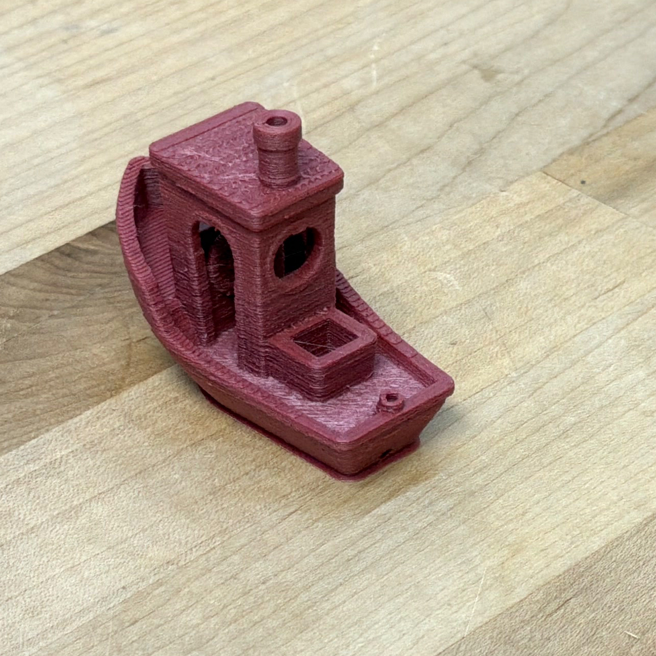
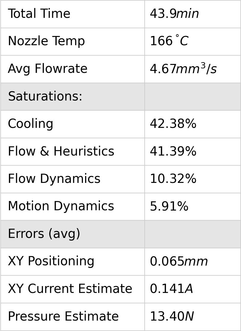
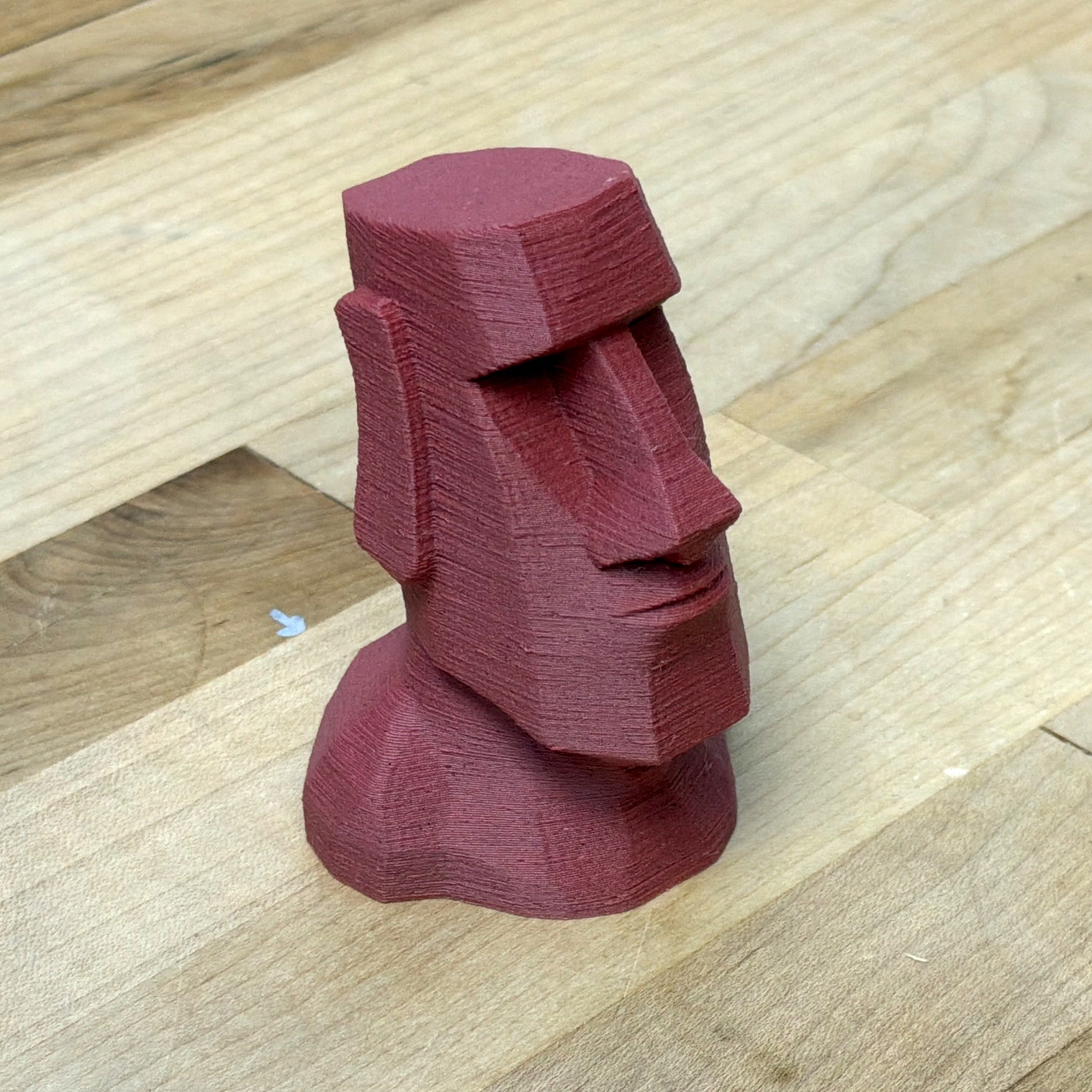
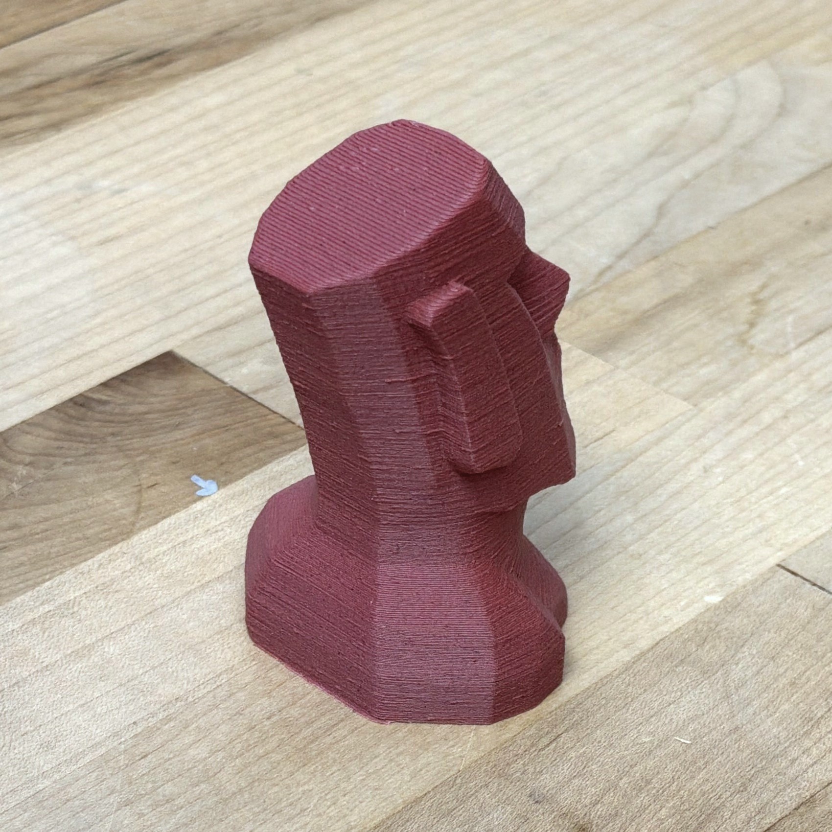
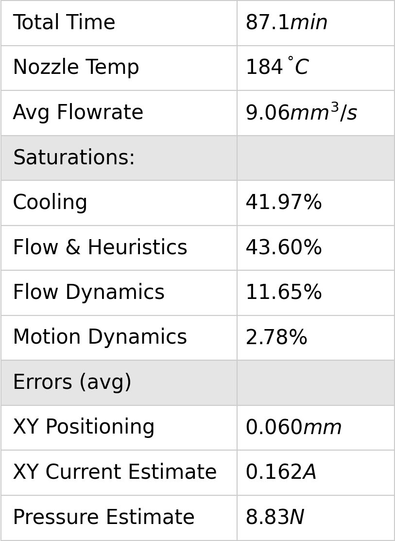
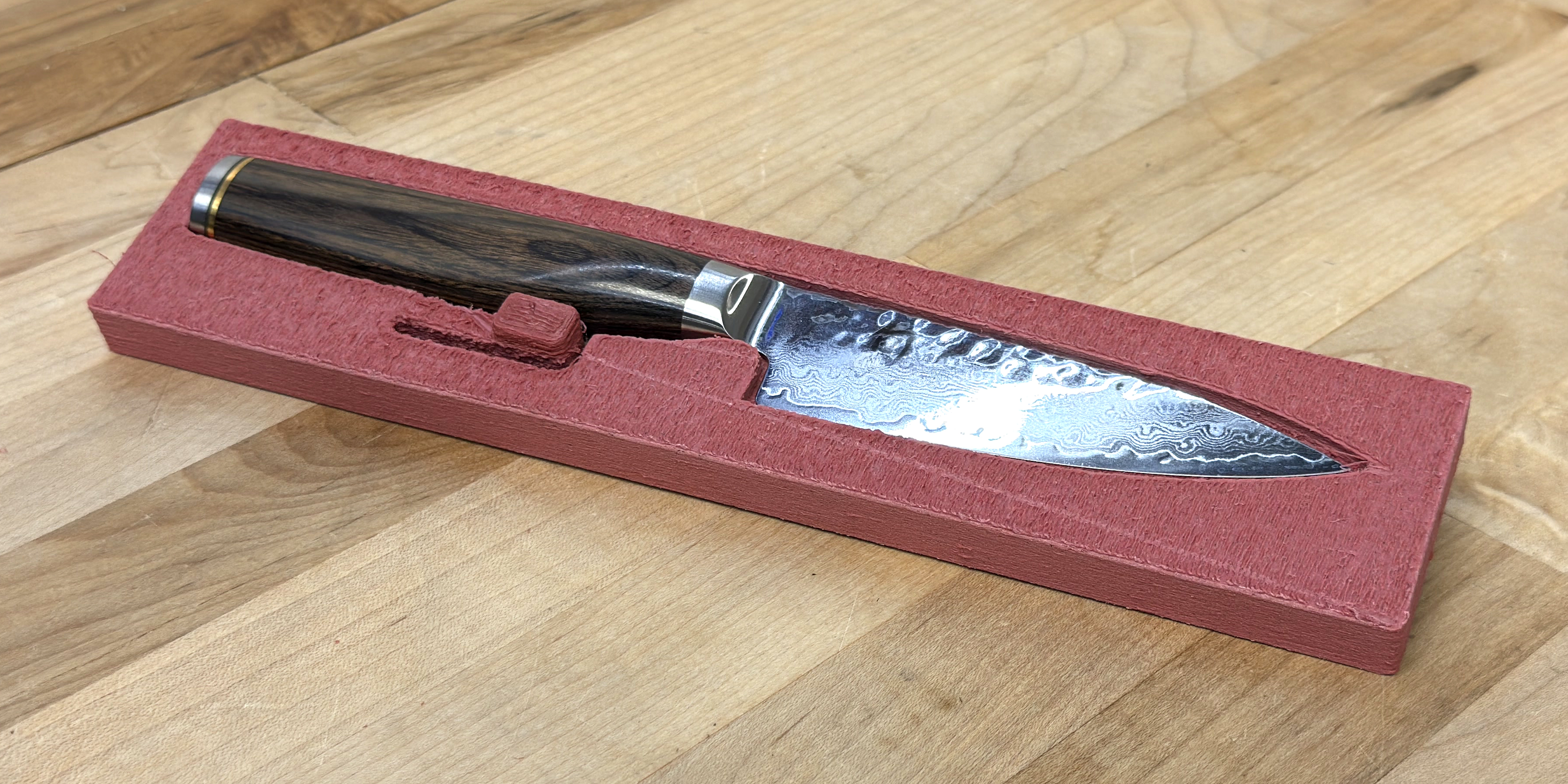
A kitchen knife case in TimerFill, printed using a 0.4mm High Flow Nozzle.
Geometry was mistakenly generated for a 0.6mm Nozzle.
Geometry was mistakenly generated for a 0.6mm Nozzle.
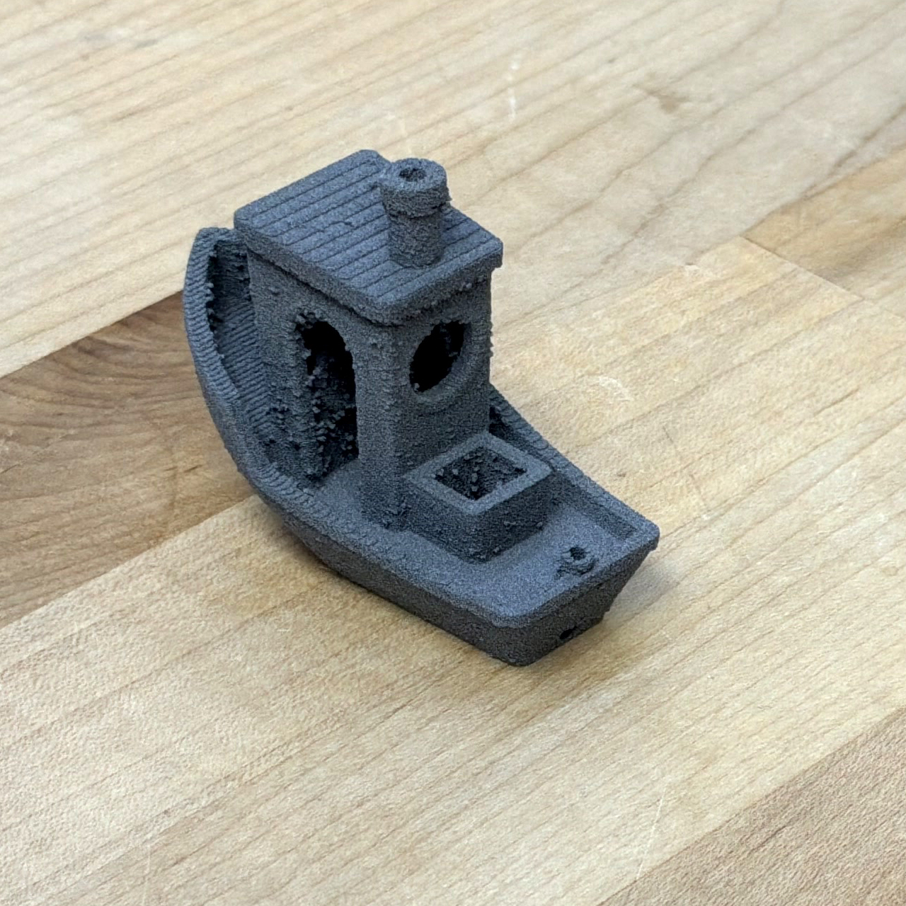
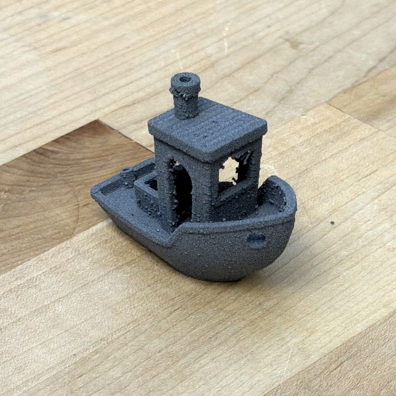
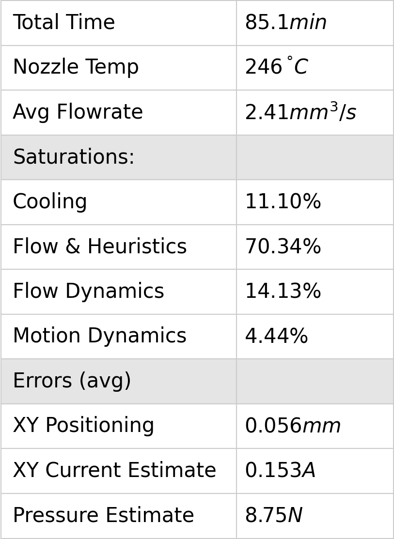
AluFill (67 percent, unknown binder), 0.6mm High Flow Coated, Benchy, Stepper Circuit Heatsink.
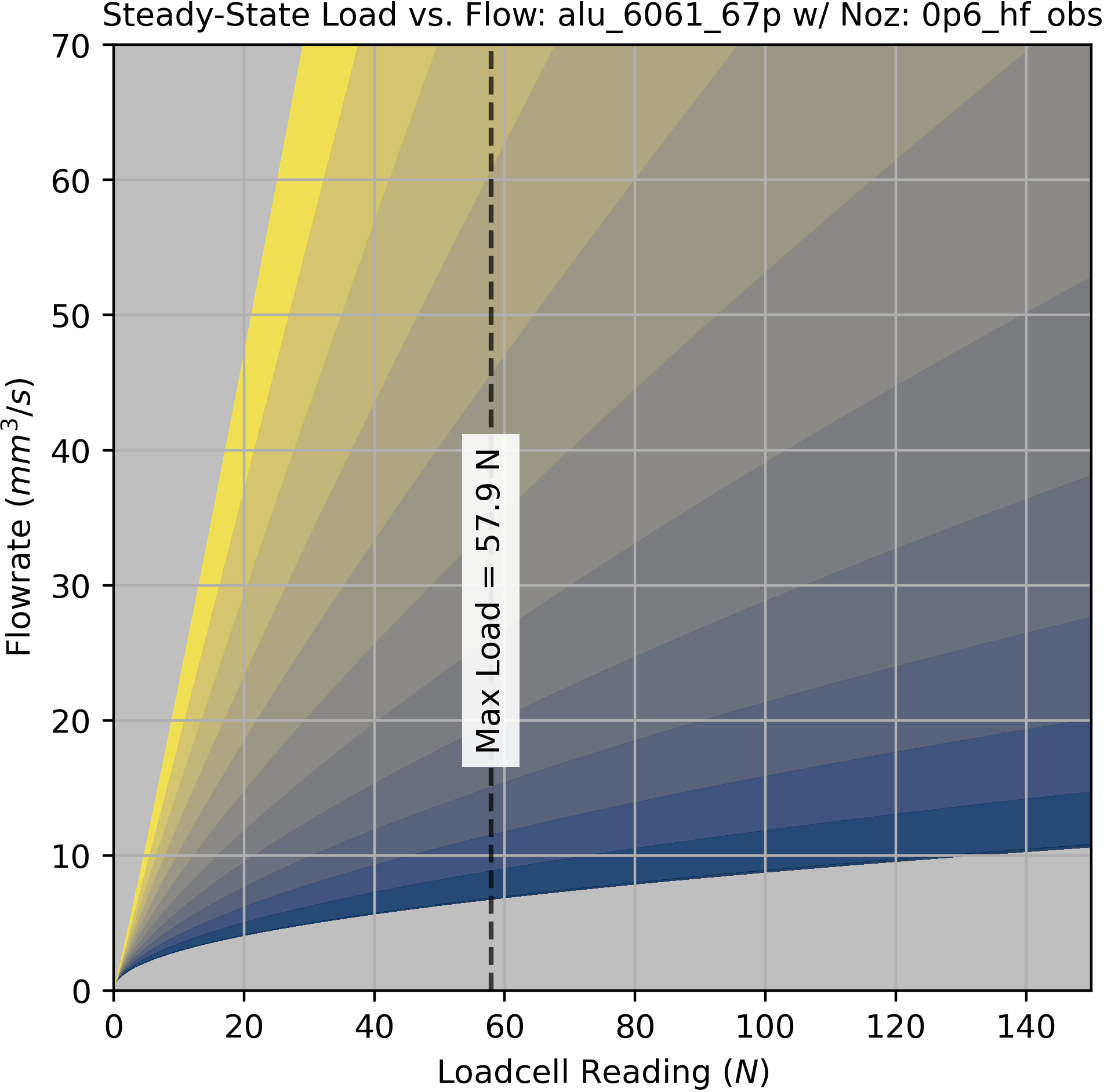
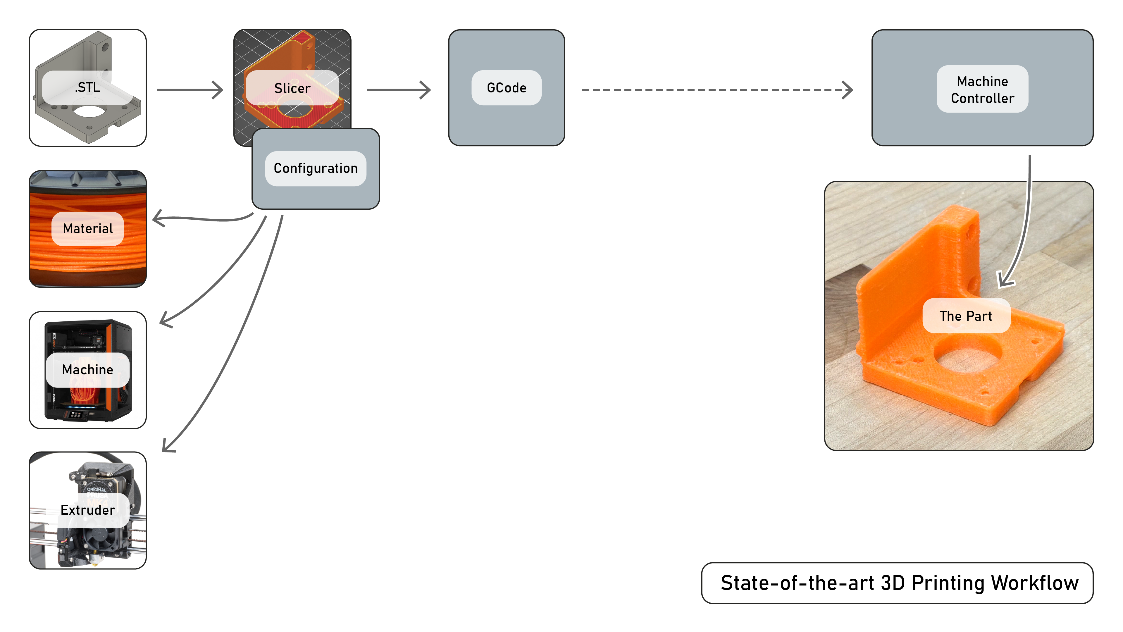
State-of-the-art workflow: manual configuration.
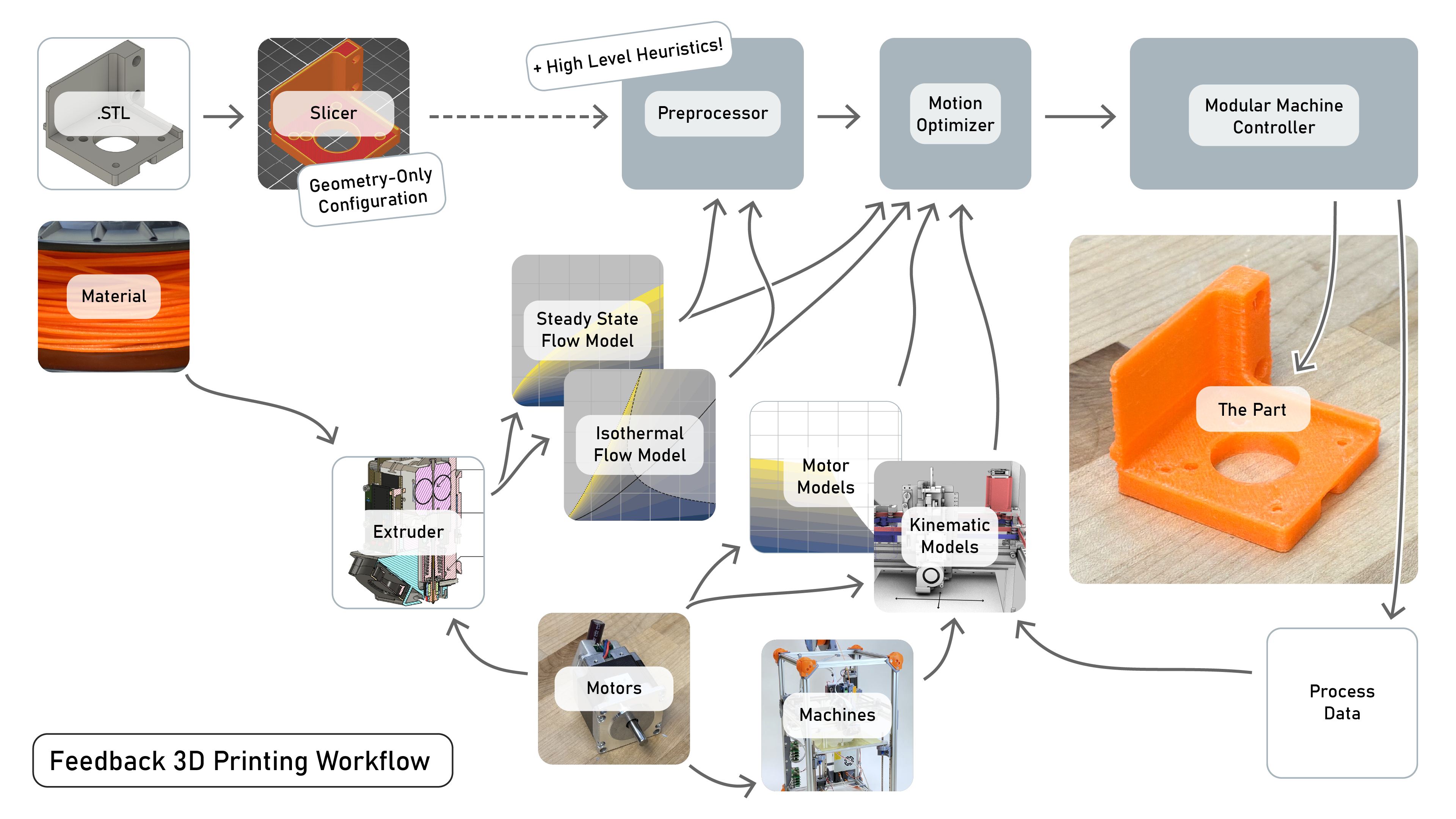
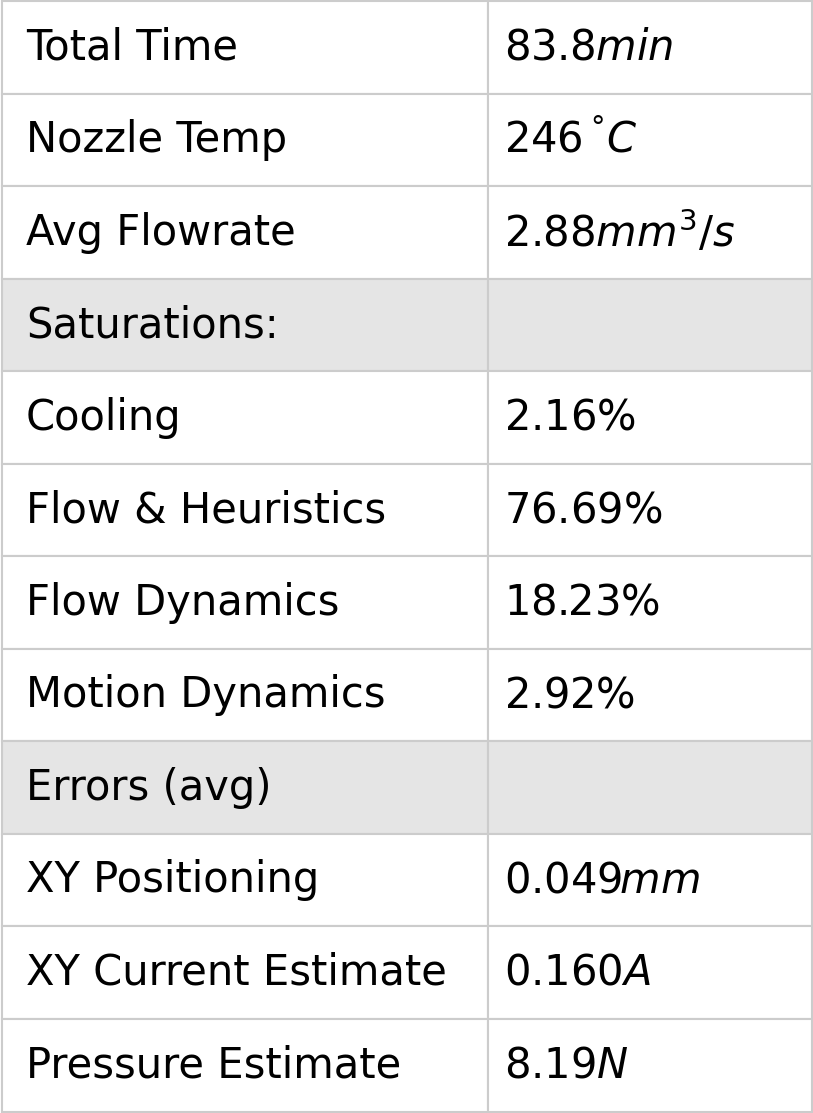
Feedback-based workflow: model-based, plus extendable heuristics.
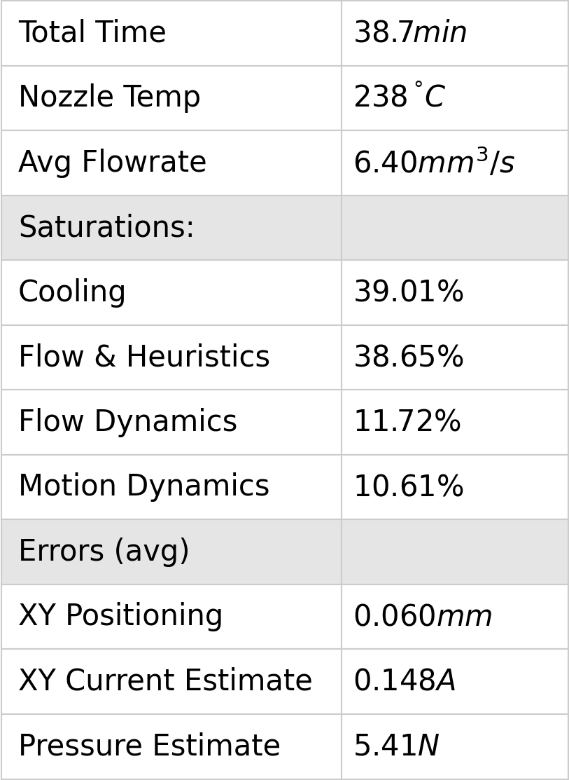
State-of-the-art workflow has ~ 47 parameters:
- 16: geometric (or functions of)
- 12: translational rates
- 7: acceleration
- 3: temperatures (nozzle, bed, chamber)
- 1: direct relation to flow (max rate)
- 4: retraction related
Per material:
- 12: translational rates
- 3: temperatures (nozzle, bed, chamber)
- 1: direct relation to flow (max rate)
- 4: retraction related
Per machine:
- 12: translational rates
- 7: acceleration
- 3: temperatures (nozzle, bed, chamber)
- 1: direct relation to flow (max rate) *
- 4: retraction related *
Feedback-based requires 21 heuristics / estimates:
- 4: cooling model estimates
- 1: first layer rate
- 1: minimum flowrate
- 3: pressure scalars (infill, perimeters, details)
- 8: motion scalars $(I_{prop})$
- 4: extruder heuristics
These can be broadcast across materials, by combining heuristics with models.
Per material or nozzle change:
- one flow test (~ 20 minutes)
Per machine:
- kinematic descriptions (human authorship!)*
- motor tests (n motors, ~ 15 min. each)
- axes kinematic fits (n axes, ~ 15 min. each)
- heater calibrations*
- loadcell calibration*
How to compare performance of ours vs. the state-of-the-art?
It would be difficult to make a comparison of the controllers where the underlying constraints are so varied.
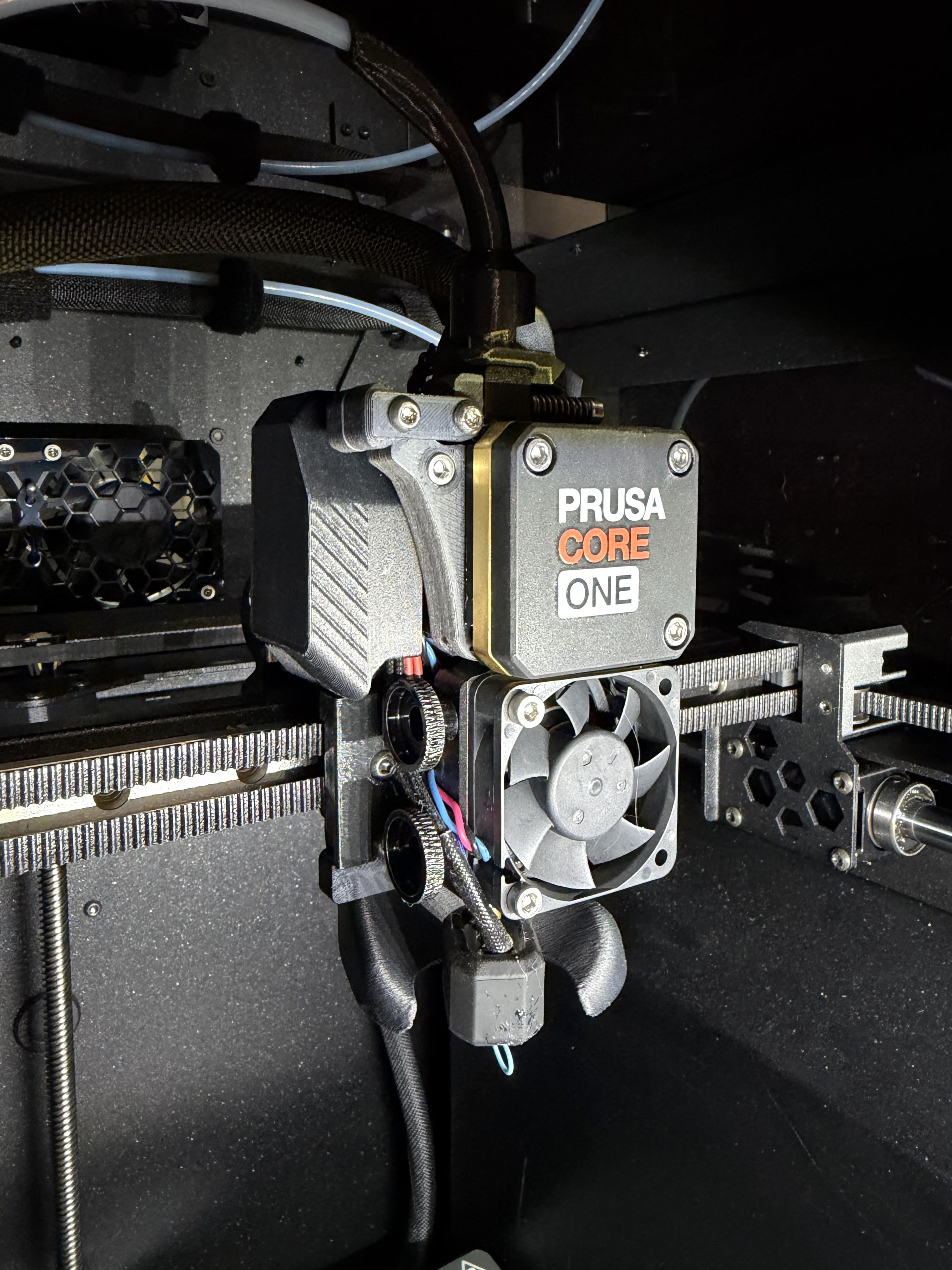
A state-of-the-art extruder, from the Prusa Core One.
The RheoPrinter Extruder
So, let's put our controllers on the state-of-the-art hardware.
A state-of-the-art extruder, from the Prusa Core One.
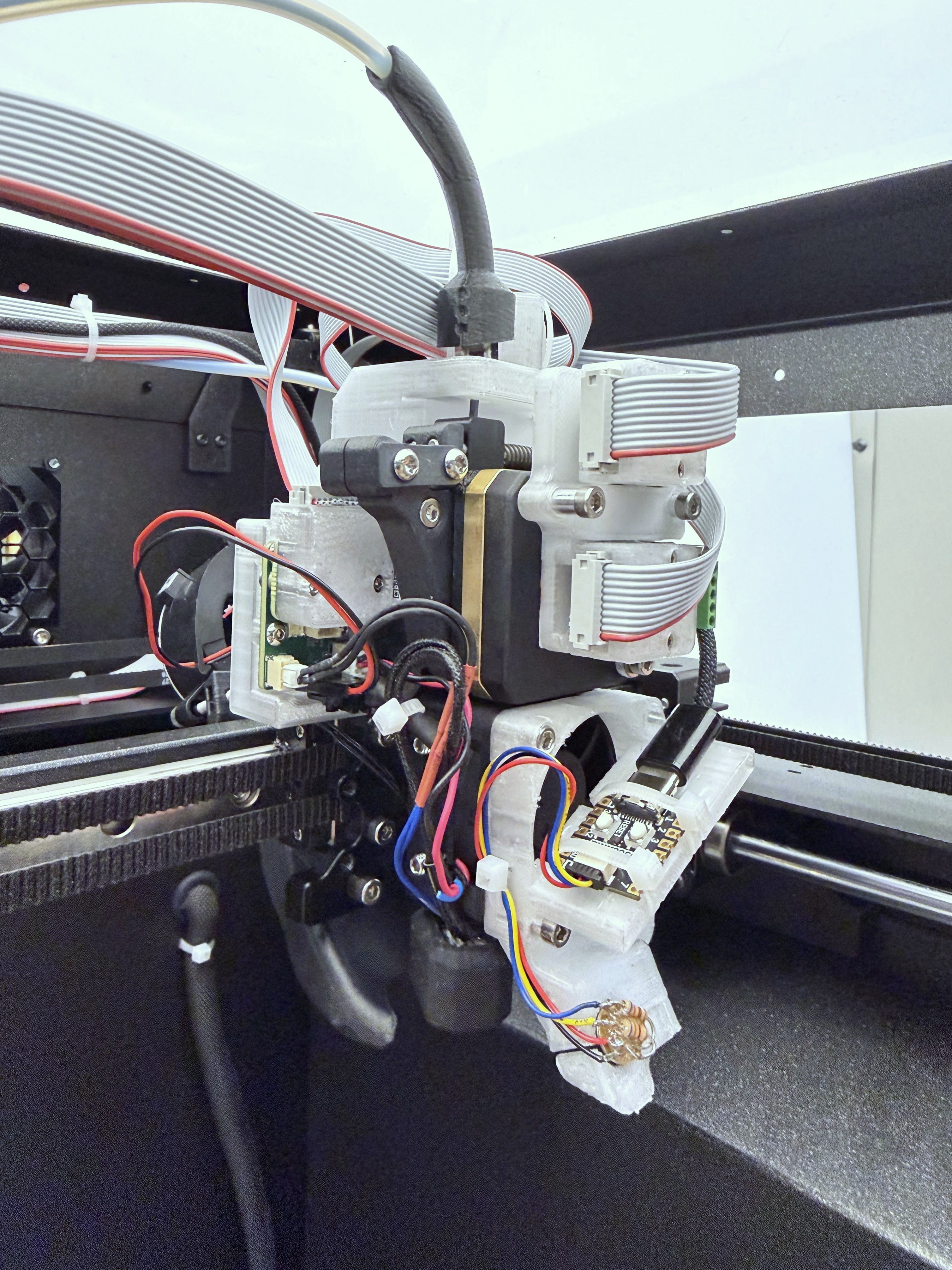
The FrankenPrusa extruder.
Prusa integrated a loadcell in their hotend for bed probing. We can piggyback on
that for our flow models.
A state-of-the-art extruder, from the Prusa Core One.
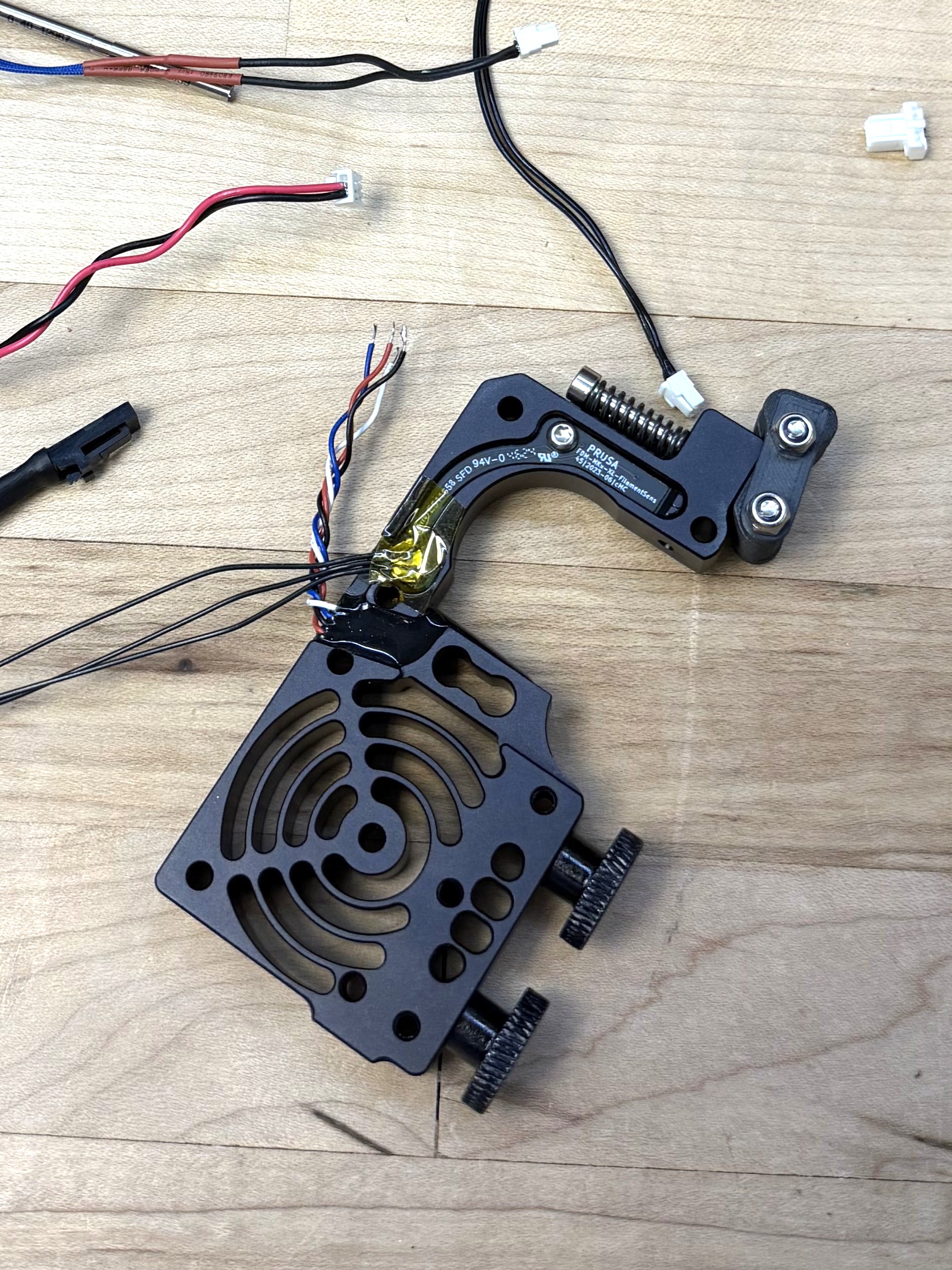
The Prusa Nextruder's integrated heatsink / loadcell.
Is it actually any faster?
| Material | Nozzle | Geometry | Total Vol. | Our Time | SOTA Time | Speedup |
| :--- | :--- | :--- | ---: | ---: | ---: | ---: |
| | | | $mm^3$ | $min.$ | $min.$ | $\\%$ |
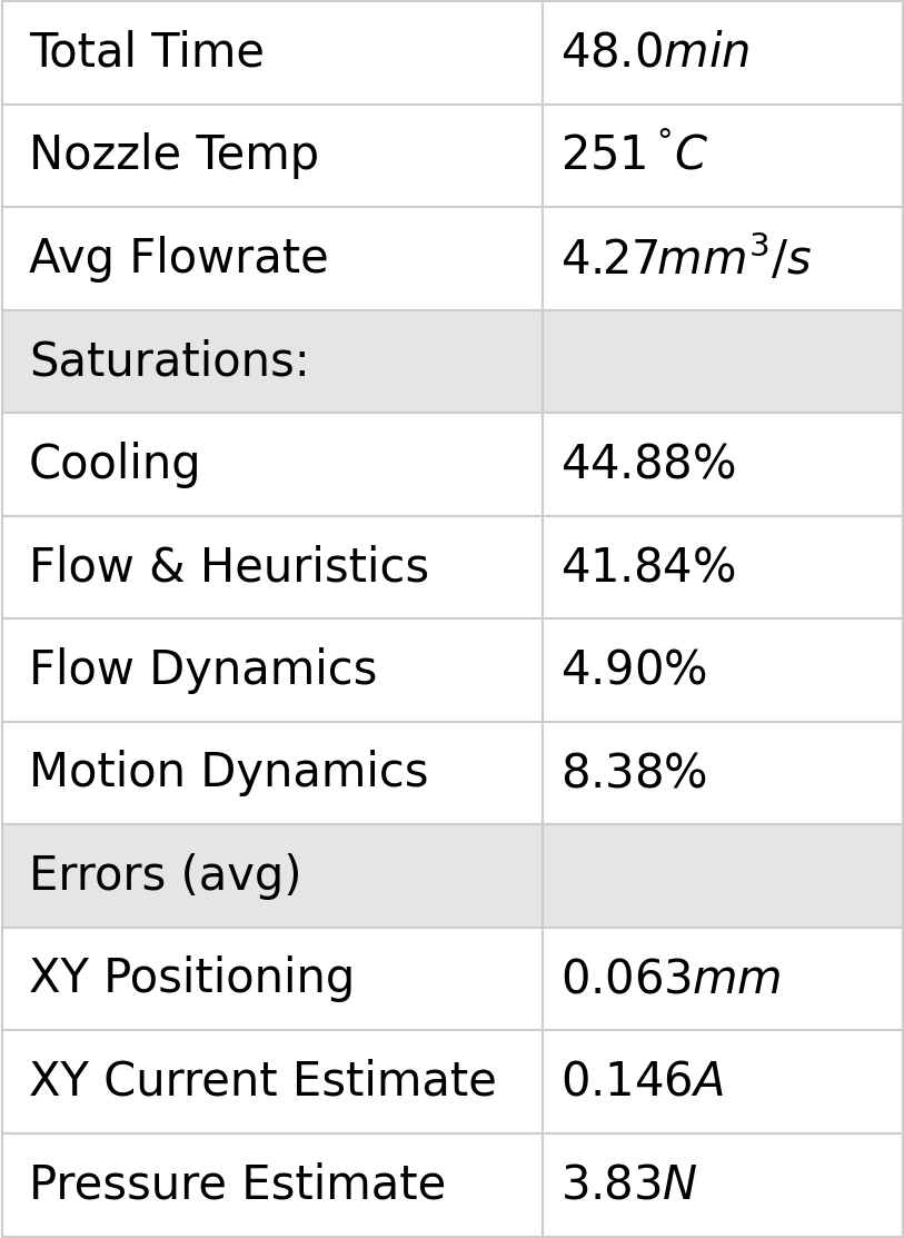
| PLA | 0.6 | 3DBenchy | 12773 | 48.0 | 53.0 | 110.4 |
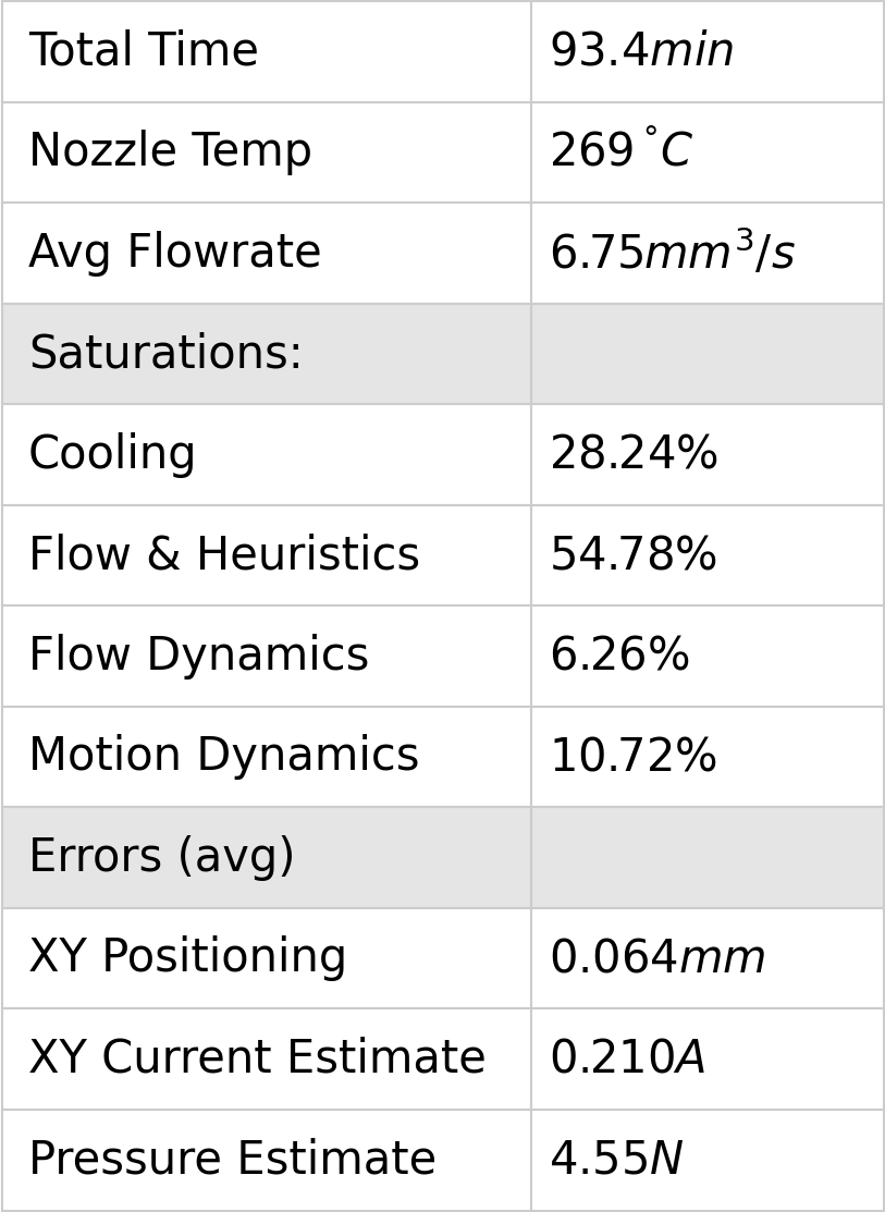
| PLA | 0.6 | 3DBenchy 1.50x | 39737 | 93.4 | 104.0 | 113.5 |
| PETG | 0.6 | 3DBenchy | 12773 | 35.3 | 58.0 | 164.3 |
| PETG | 0.6 | Roadballs | 34687 | 49.3 | 68.0 | 137.9 |
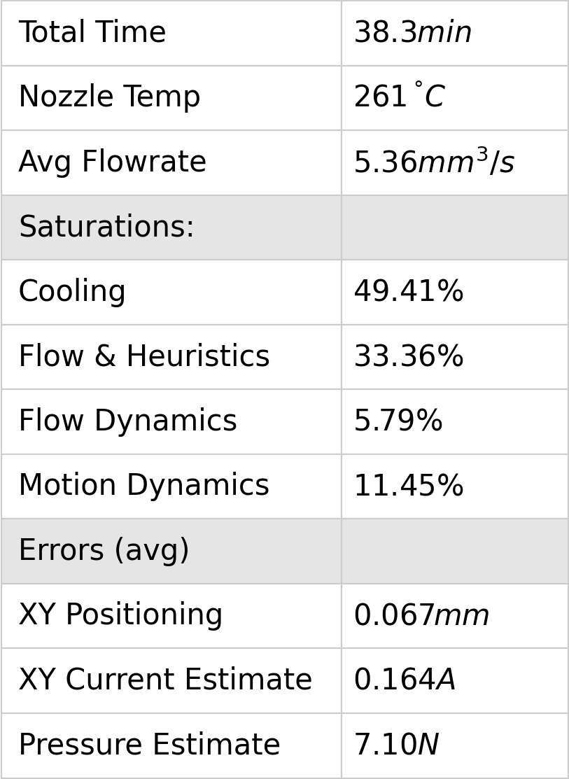
| PCBlend CF | 0.6 HF | 3DBenchy | 13125 | 38.3 | 67.0 | 175.0 |
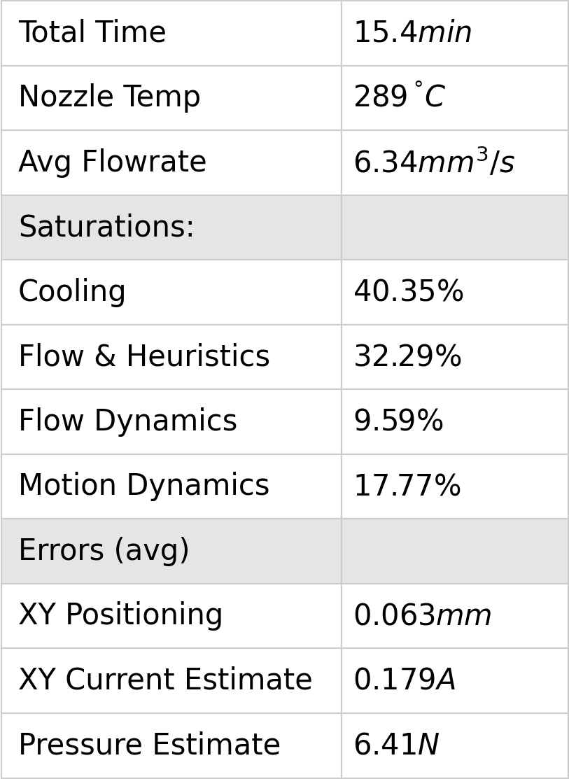
| PCBlend CF | 0.6 HF | Drone Fuselage Cap | 6119 | 15.4 | 23.0 | 149.4 |
| PCBlend CF | 0.6 HF | Drone Arms | 32247 | 60.4 | 80.0 | 132.5 |
| PCBlend CF | 0.6 HF | Drone Fuselage Halves | 42233 | 65.1 | 92.0 | 141.3 |
The workflow developed here increases speed over the state-of-the-art workflow
over this set of prints by $141 \%$ on average.
over this set of prints by $141 \%$ on average.
What about the quality of our parts?
PLA, 0.6mm Brass Nozzle, Benchy SOTA (left) vs. Ours
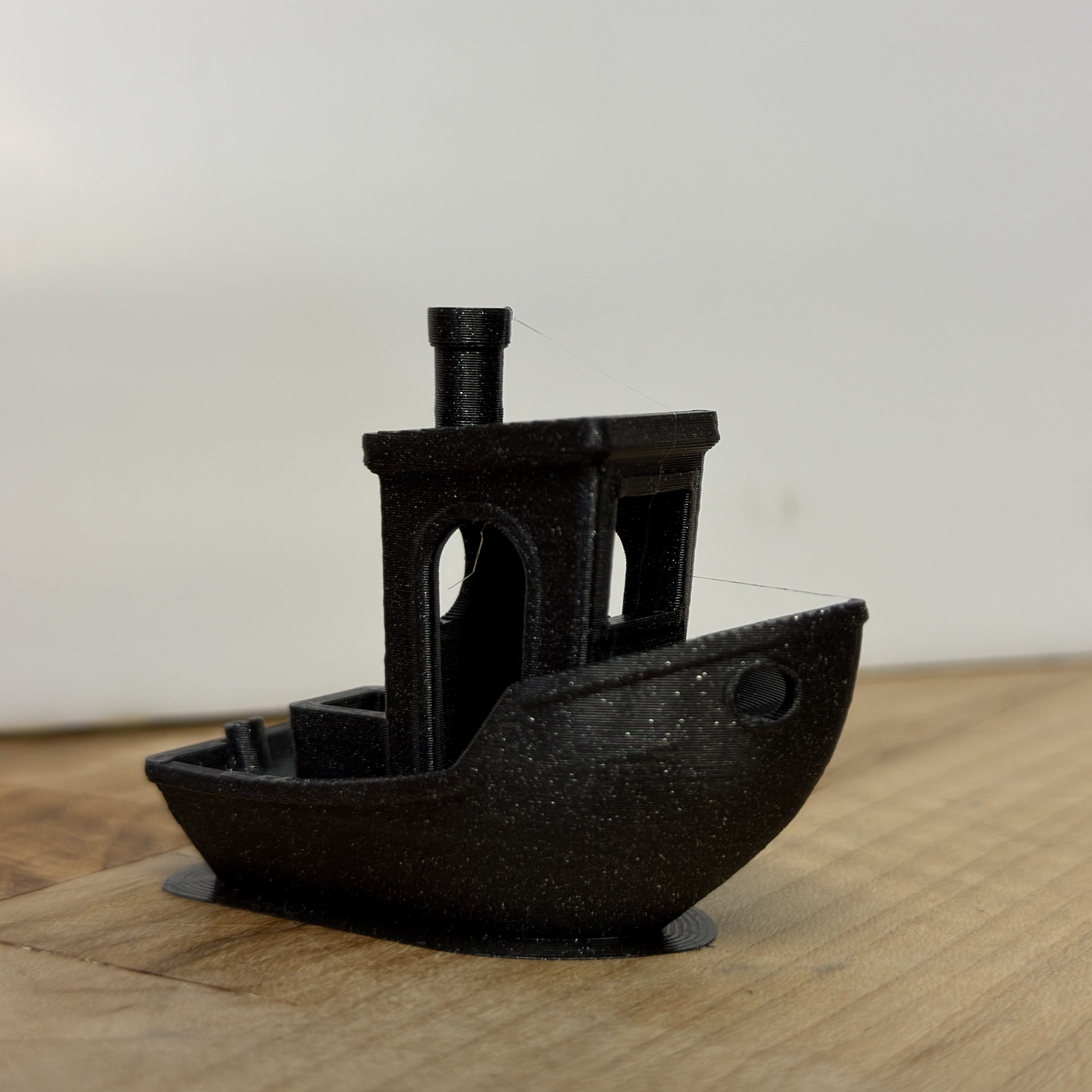
SOTA
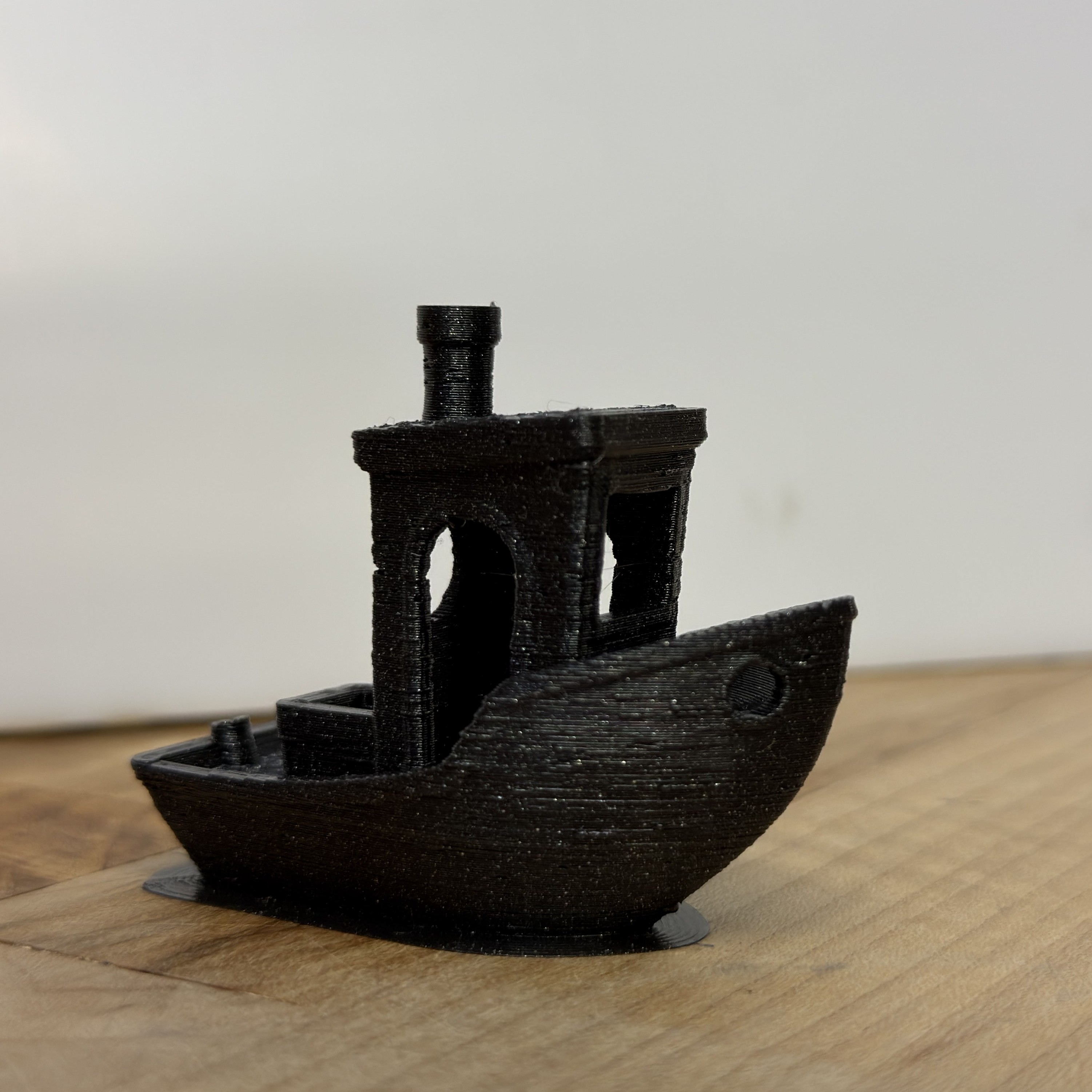
Ours
PETG, 0.6mm Brass Nozzle, Benchy SOTA (left) vs. Ours
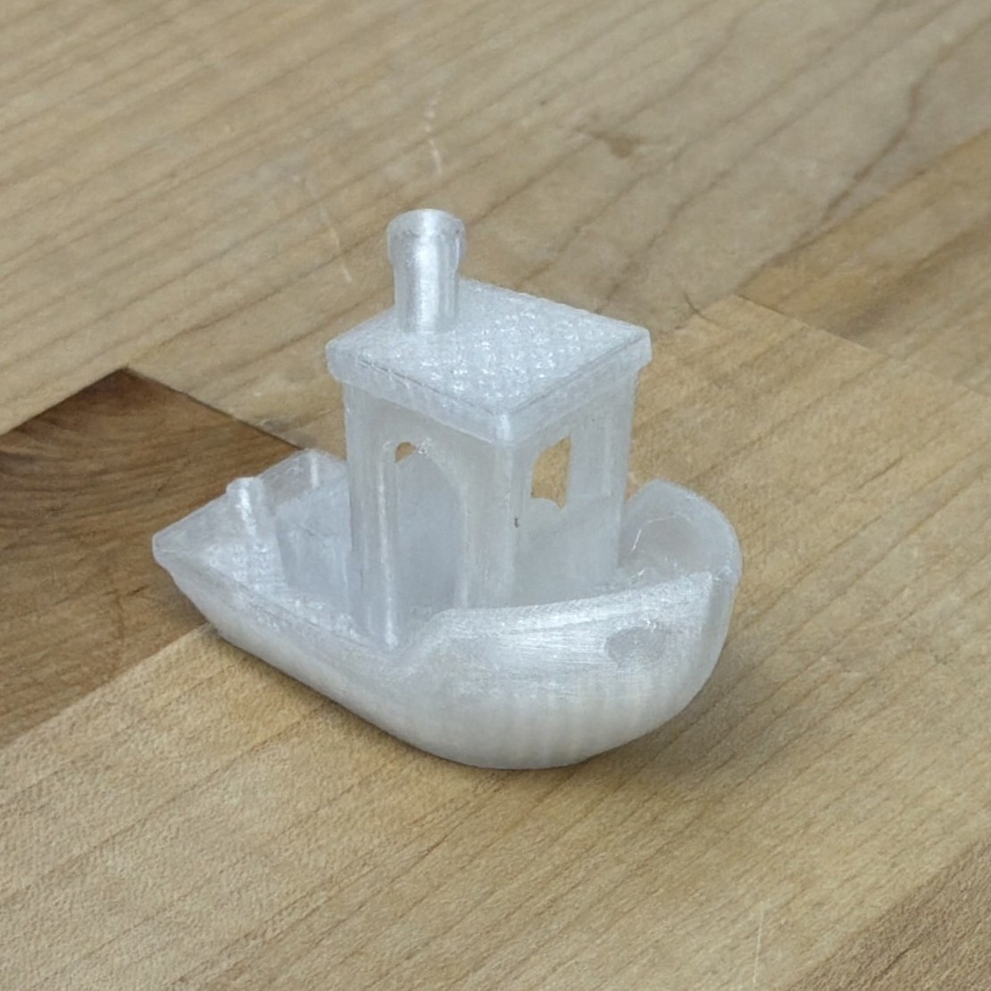
SOTA
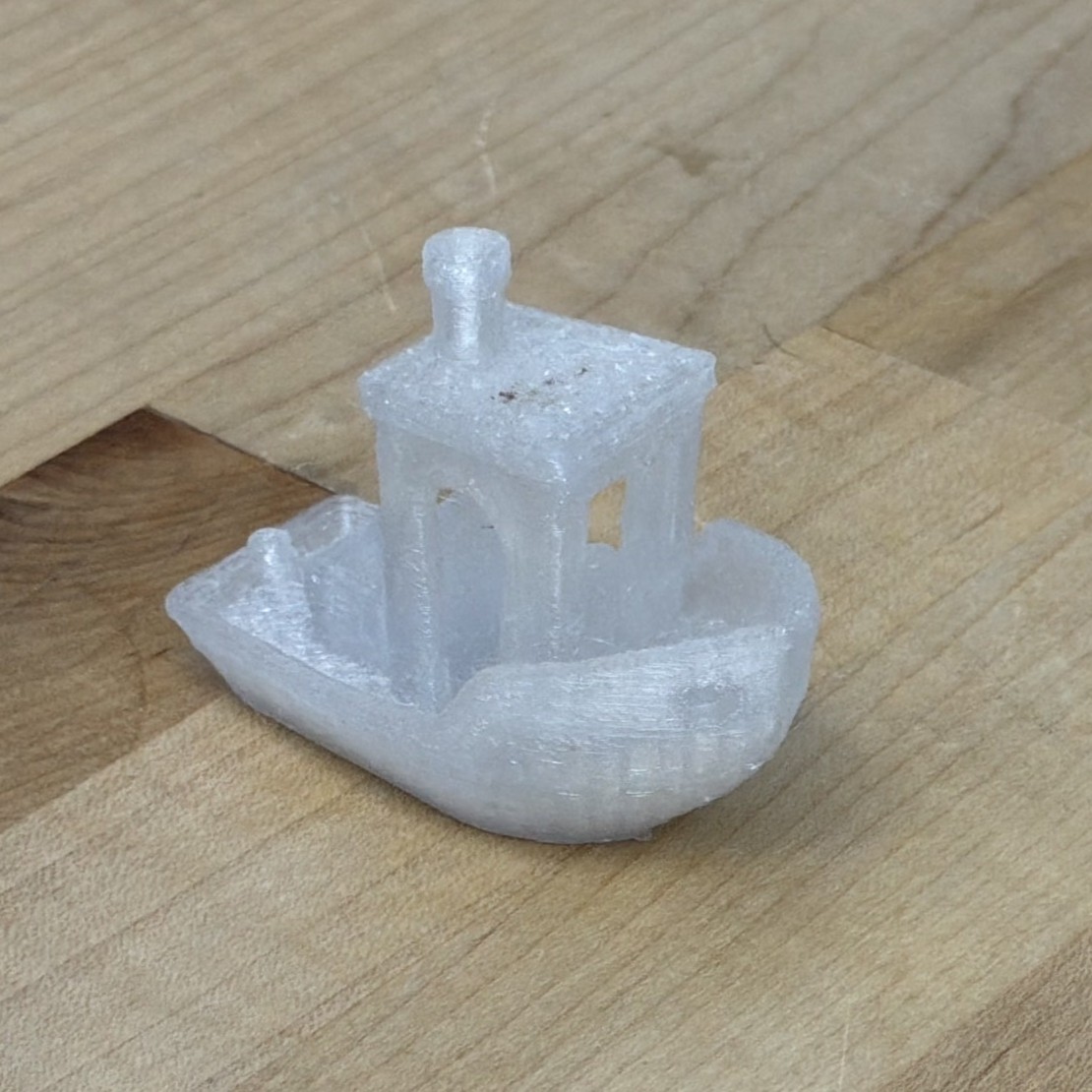
Ours
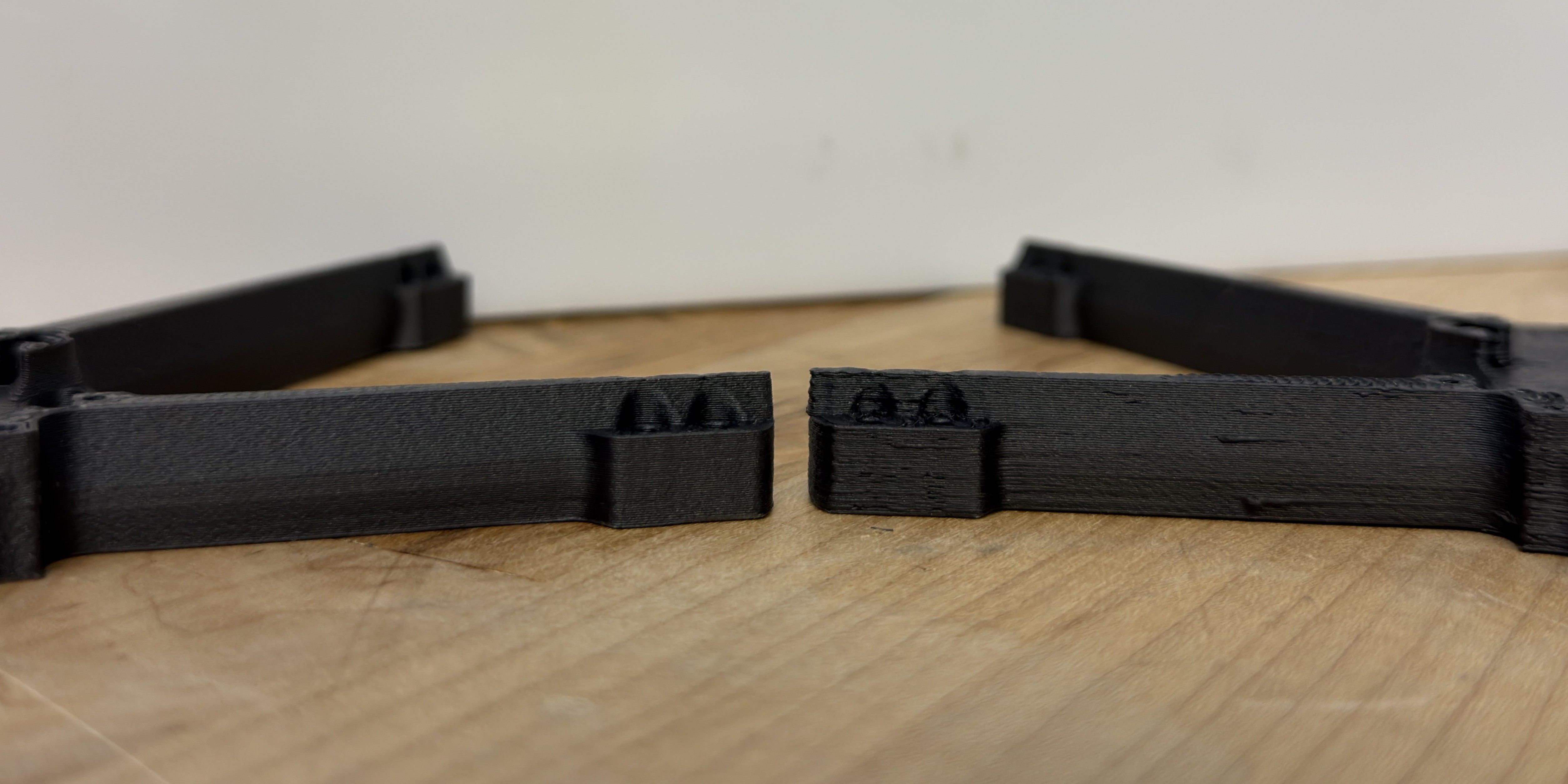
PCBlend, 0.6mm High Flow Coated Nozzle,
Drone Arms SOTA vs. Ours
Drone Arms SOTA vs. Ours
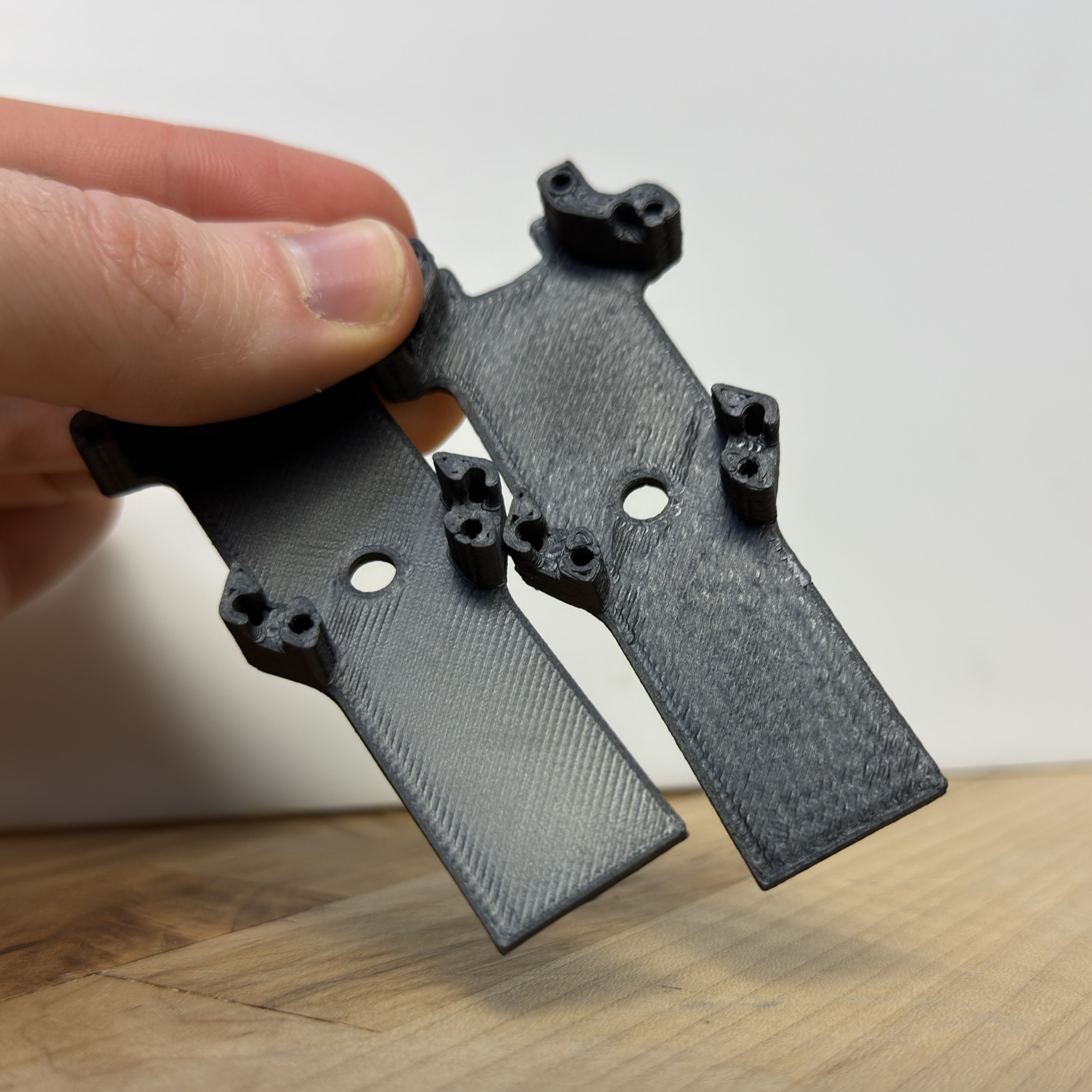
PCBlend, 0.6mm High Flow Coated Nozzle,
Drone Fuselage Cap SOTA vs. Ours
Drone Fuselage Cap SOTA vs. Ours
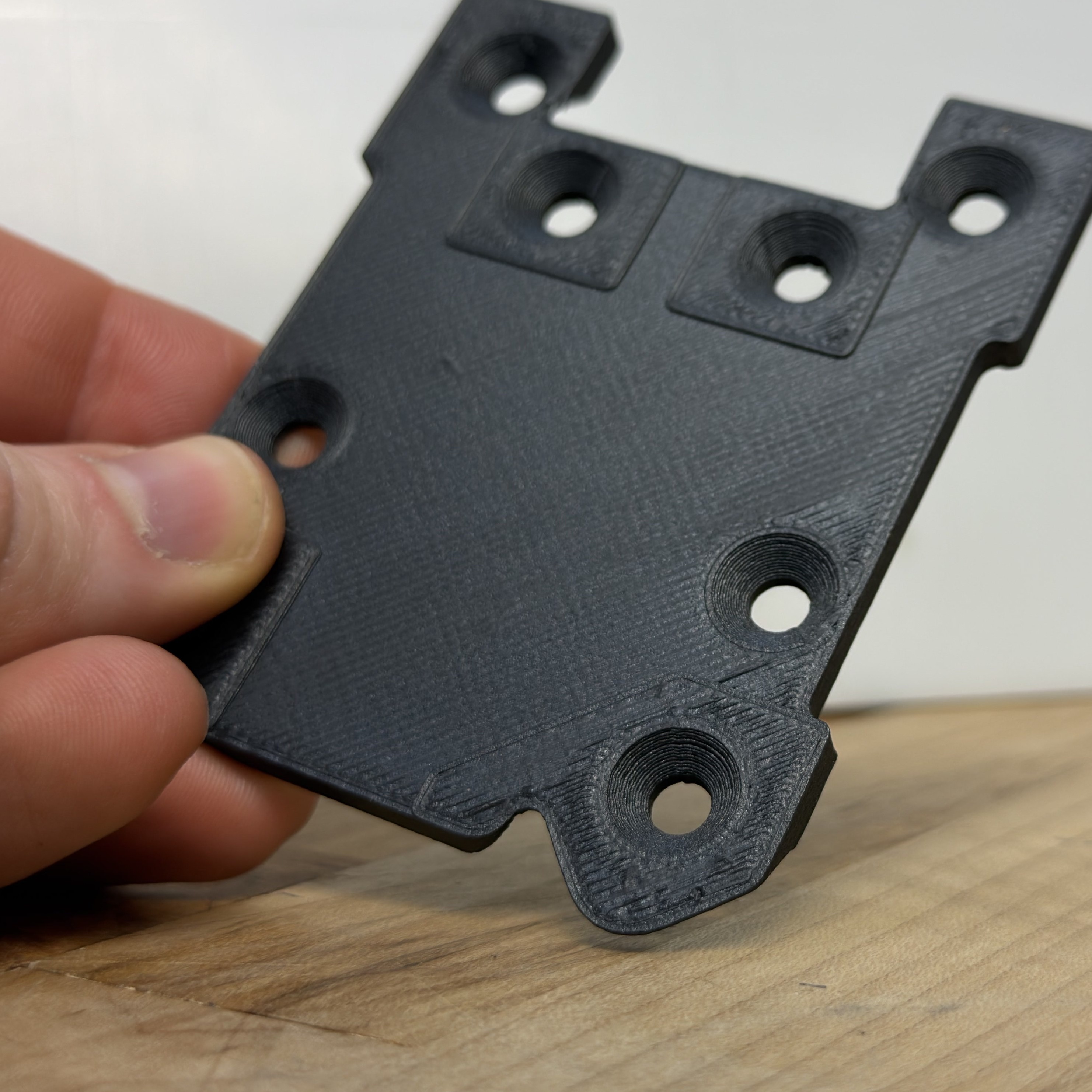
SOTA (PETG-CF, 0.4mm High Flow Nozzle)
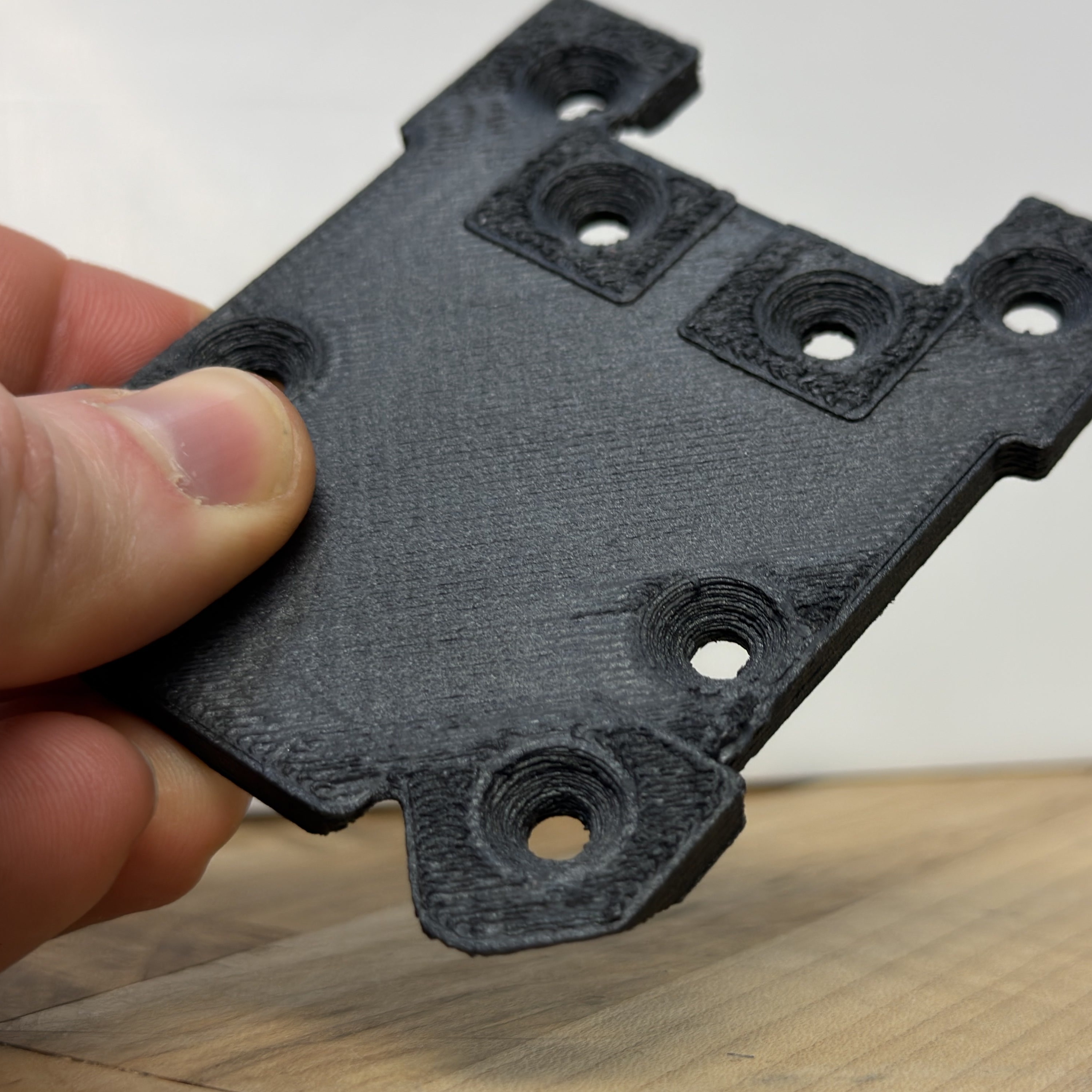
Ours (PETG-CF, 0.4mm High Flow Nozzle)
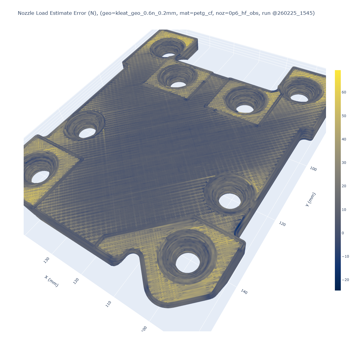
Pressure Estimate Error
$err=F_{meas}-F_{slvr} \ (N)$
$err=F_{meas}-F_{slvr} \ (N)$
Ours (PETG-CF, 0.4mm High Flow Nozzle)
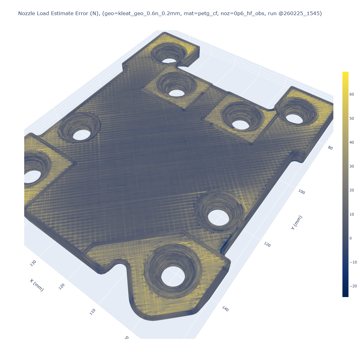
Pressure Estimate Error
$err=F_{meas}-F_{slvr} \ (N)$
$err=F_{meas}-F_{slvr} \ (N)$
High-resolution time-series from our workflow should allow us to continuously improve models.
The printer generates ~ 1GB/h of data.
The printer generates ~ 1GB/h of data.
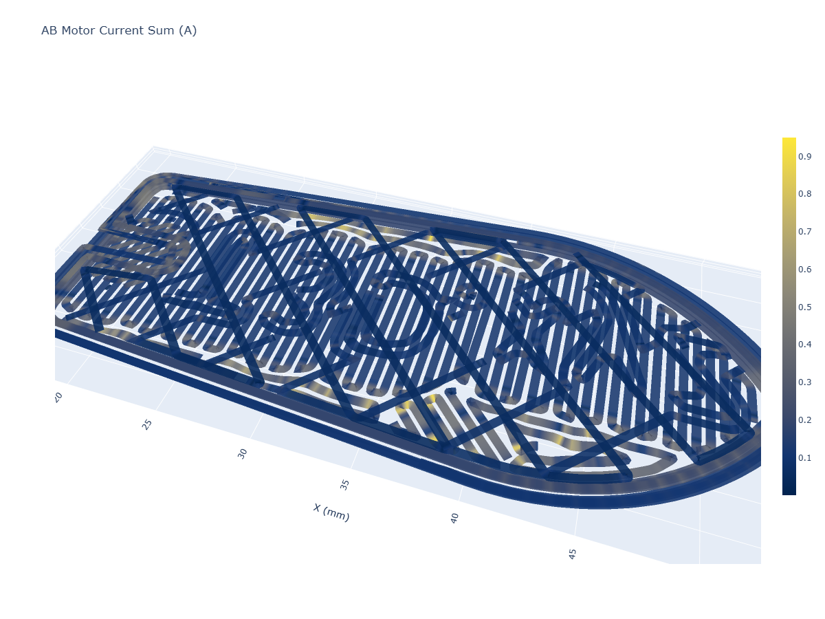
Measured Actuator Currents
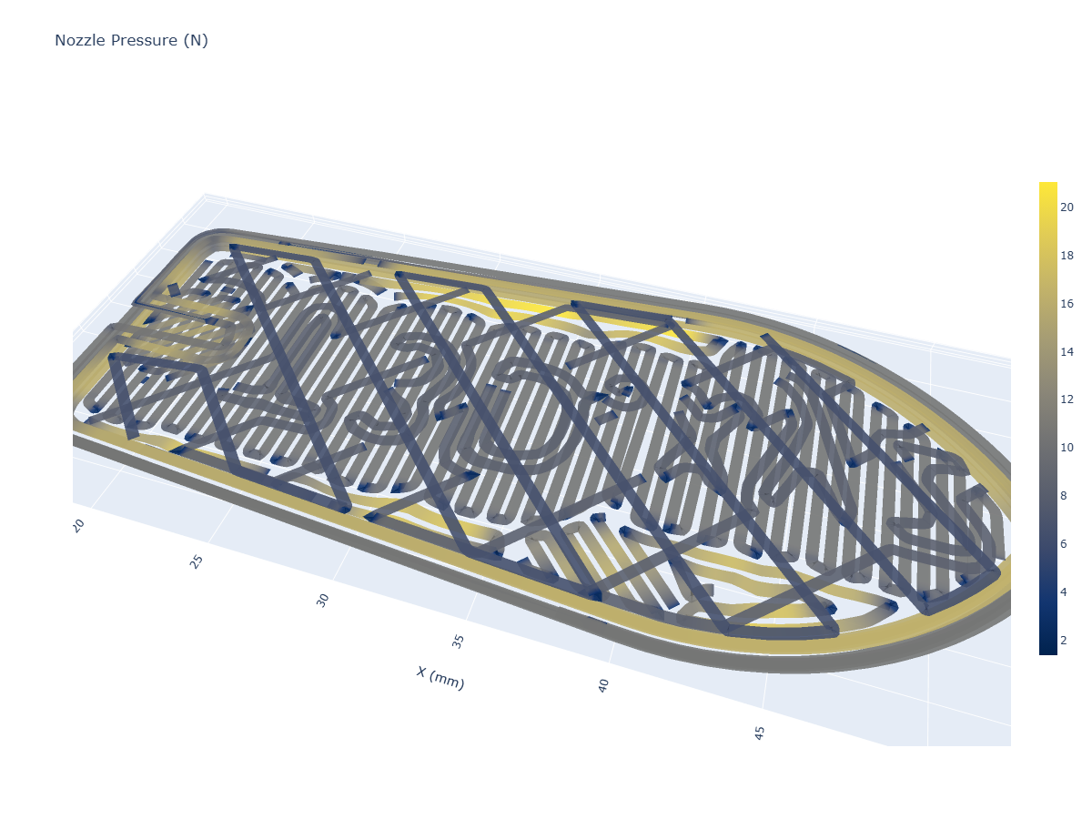
Measured Nozzle Pressure
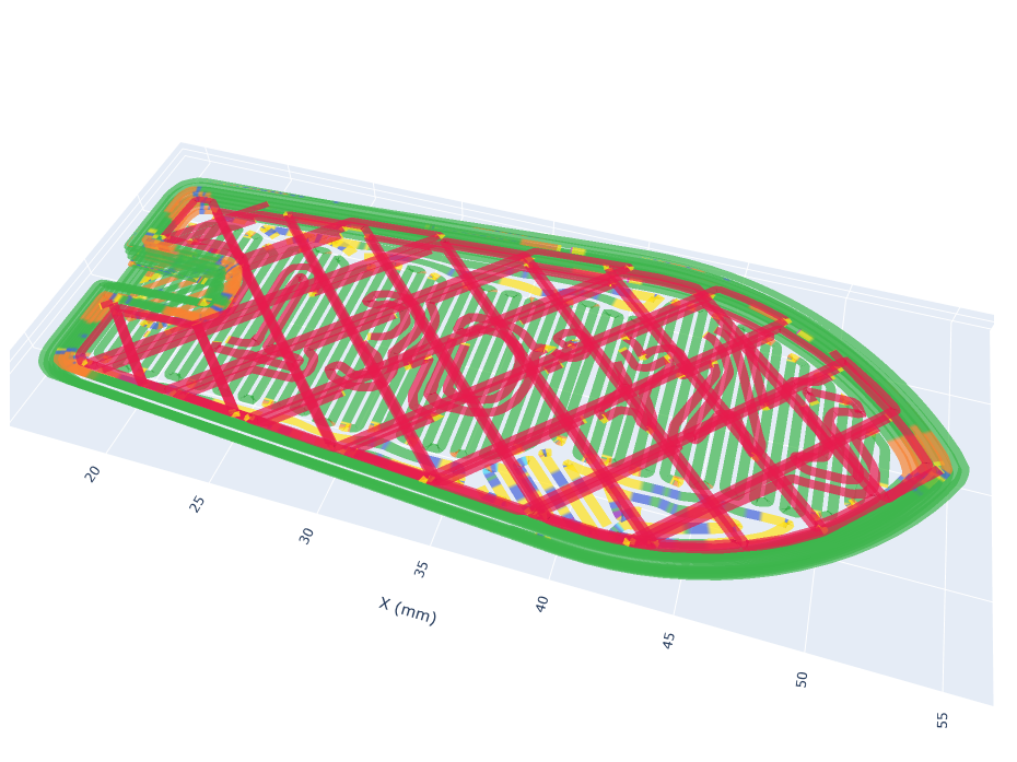
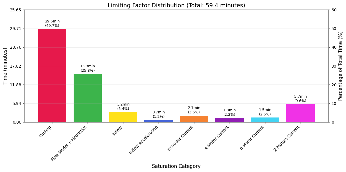
We can process solver outputs to assess which process factor was limiting overall speed.
This type of tool helps us to understand complete interactions between process control, motion control, and our part geometries and materials.
This type of tool helps us to understand complete interactions between process control, motion control, and our part geometries and materials.
I developed a time-optimal workflow for FFF that explicitly frames both high- and low-level
aspects of machine control as optimization tasks.
This reduces the parameter-tuning burden on machine users, showing how model-based machines can:
- Help us develop and deploy new materials and machines
- Help new machine users to succeed
- Support the development of tacit knowledge with real data
The time-optimal workflow is faster than the state-of-the-art, but print quality
is clearly lower.
However, I showed that areas of poor print quality are correlated with
areas where model losses are high.
If we can close the loop and re-fit flow models on machine data, we can probably drive this approach towards improvements over the state-of-the-art on all fronts.
If we can close the loop and re-fit flow models on machine data, we can probably drive this approach towards improvements over the state-of-the-art on all fronts.
How does it all go together?
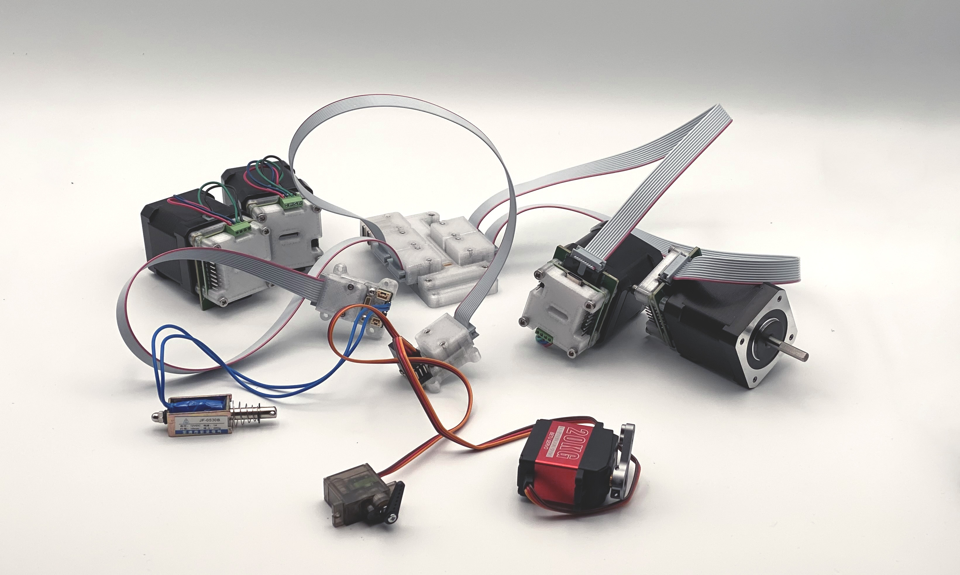
Modular circuits help to assemble machines from a core set of parts.
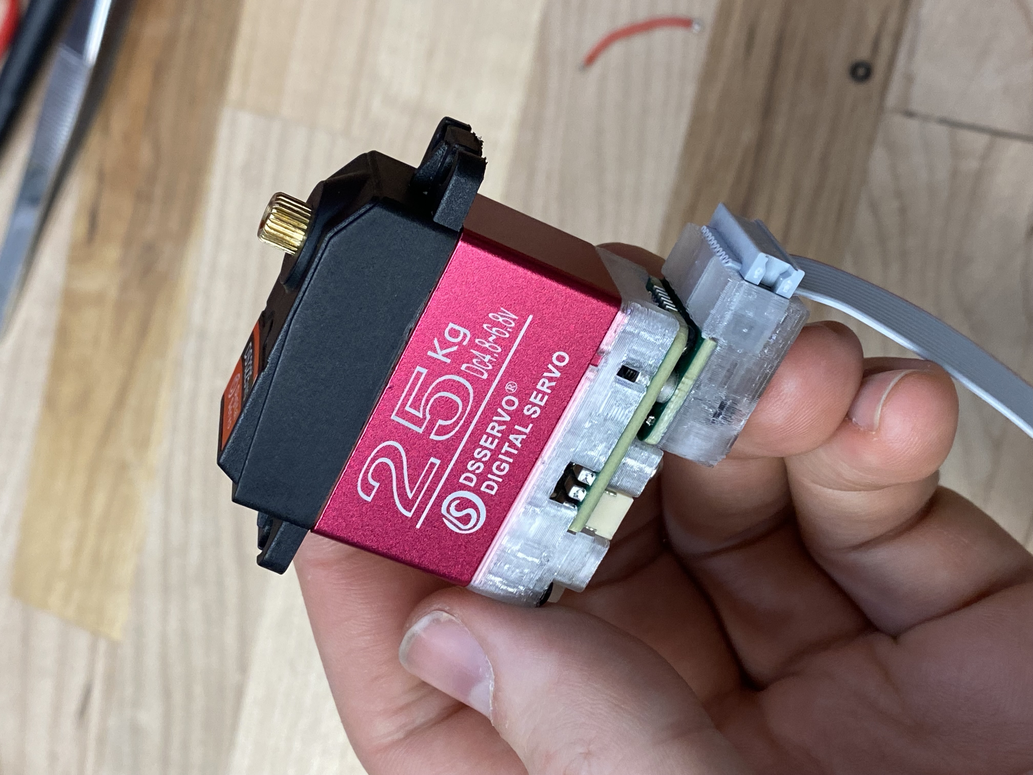
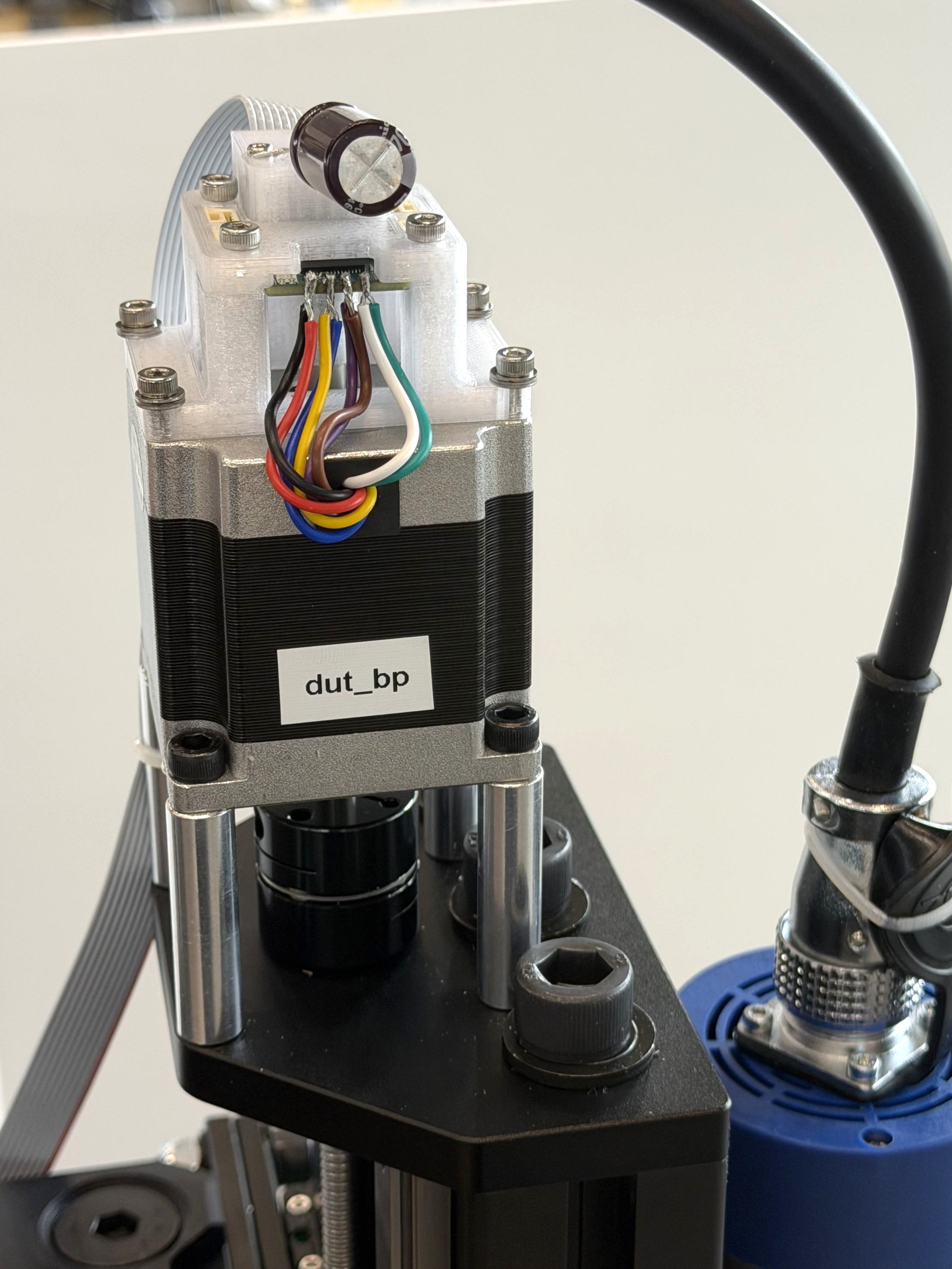
Milling Machine, Z-Axis Motor
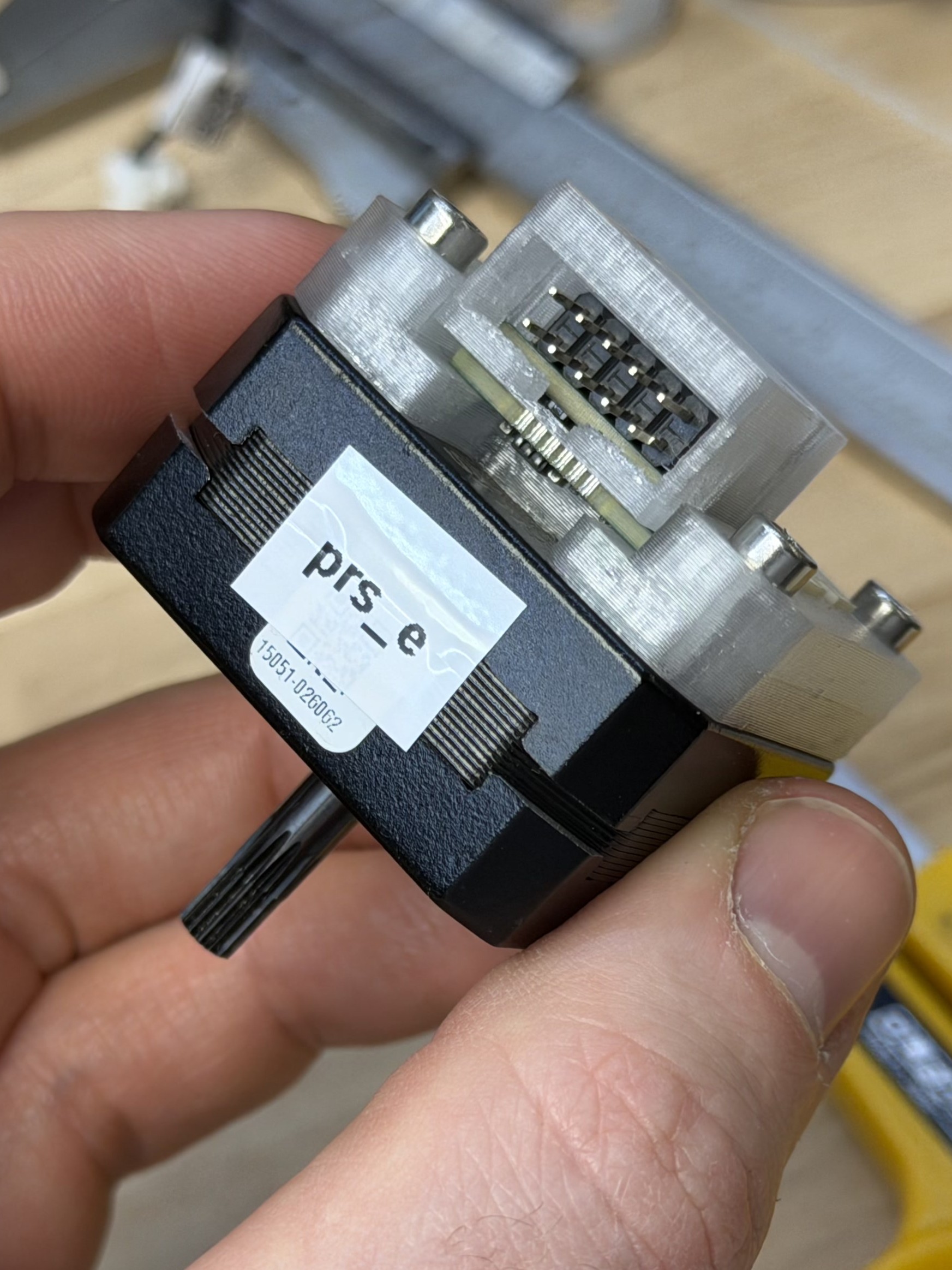
FrankenPrusa, Extruder Motor
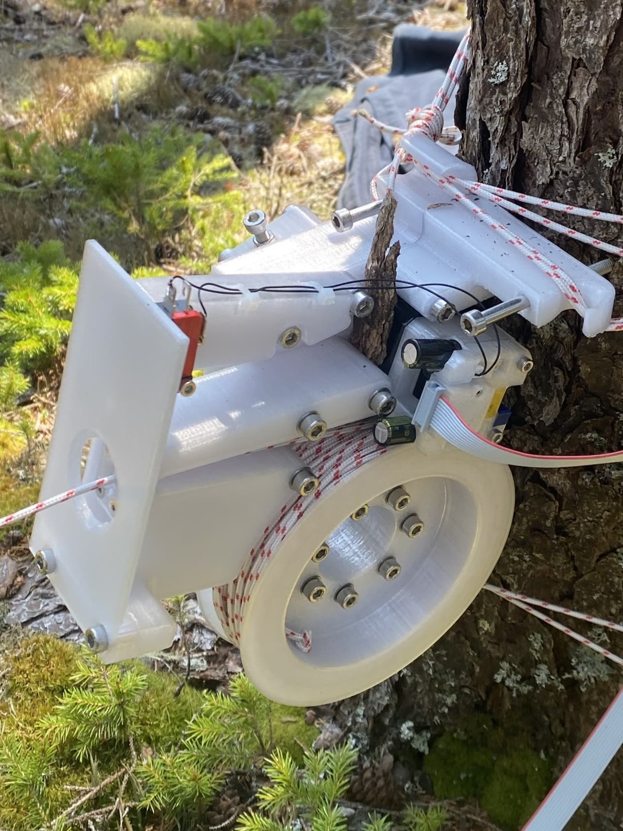
In a CNC Winch.
The FrankenPrusa is a neat opportunity to compare: monolithic vs. modular.
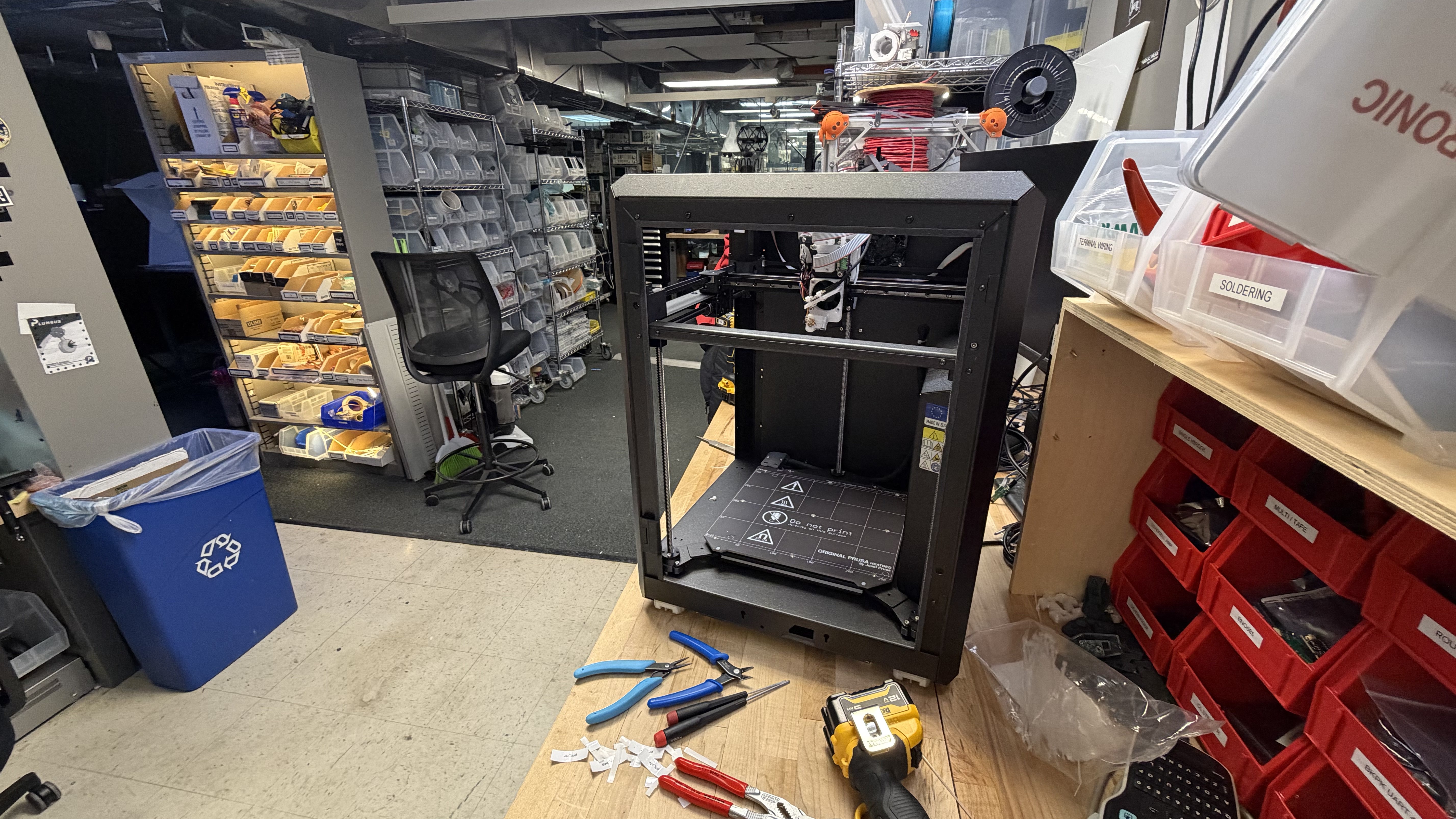
Monolithic controllers (left) vs. modular (right).
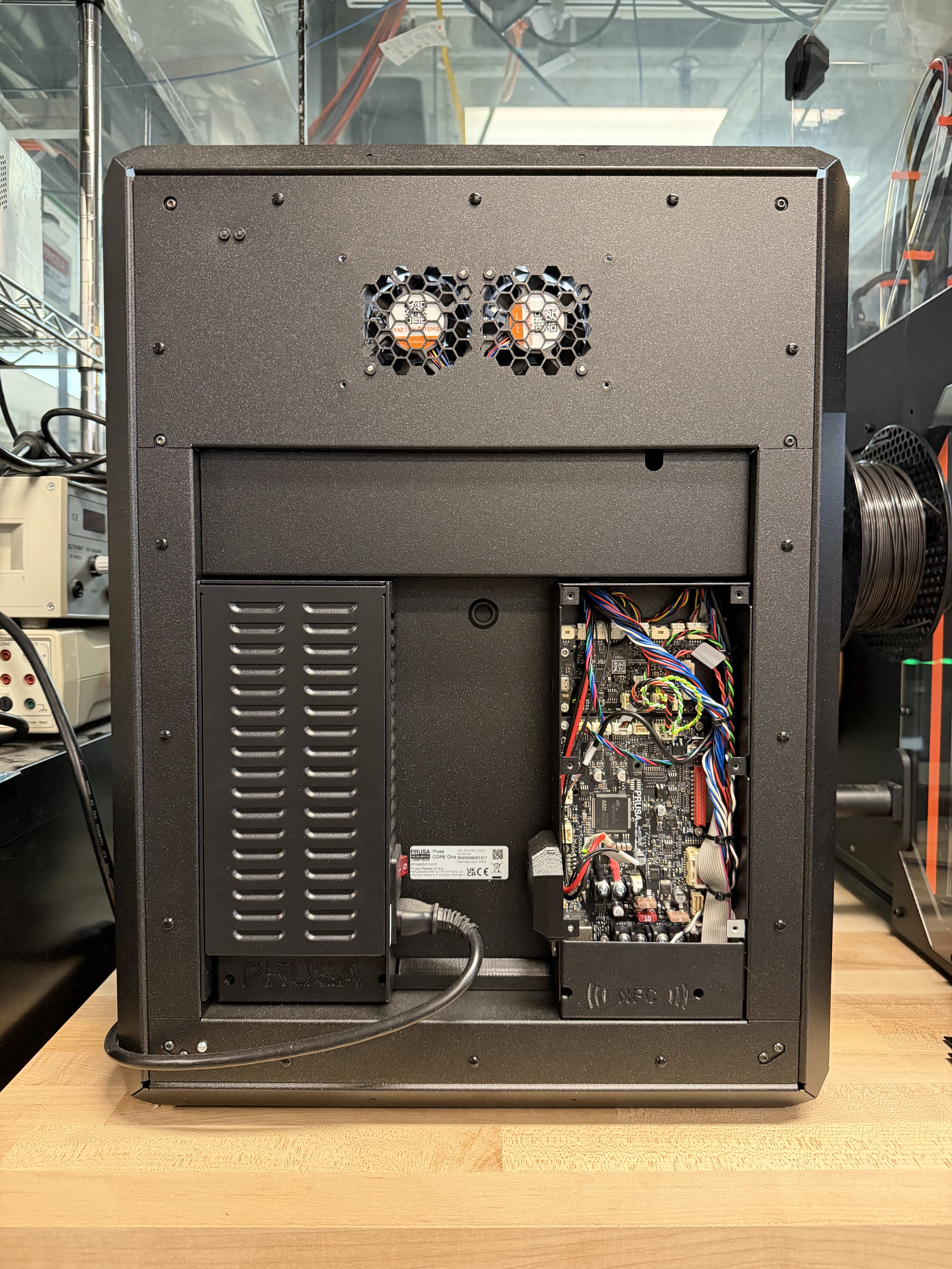
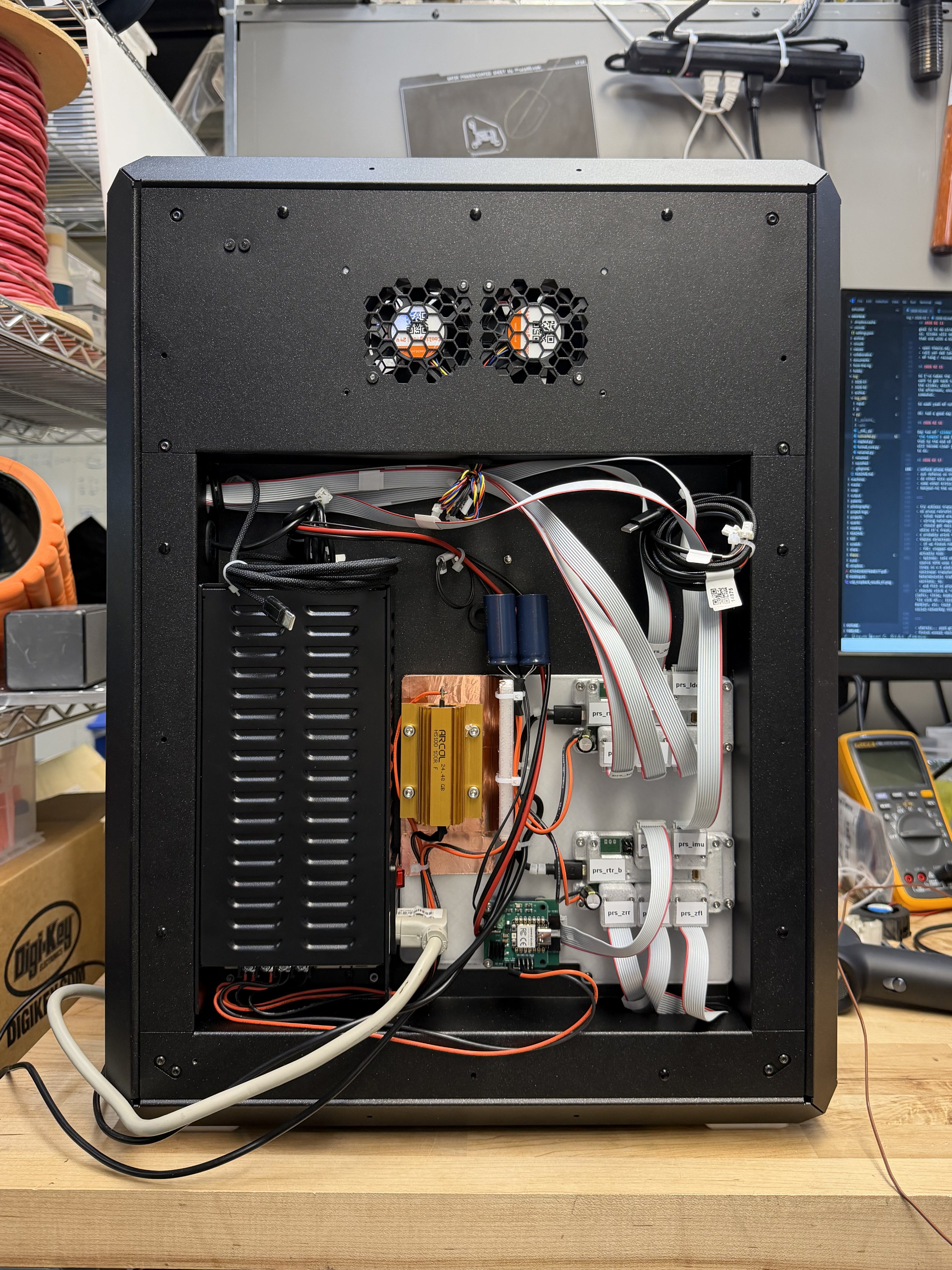
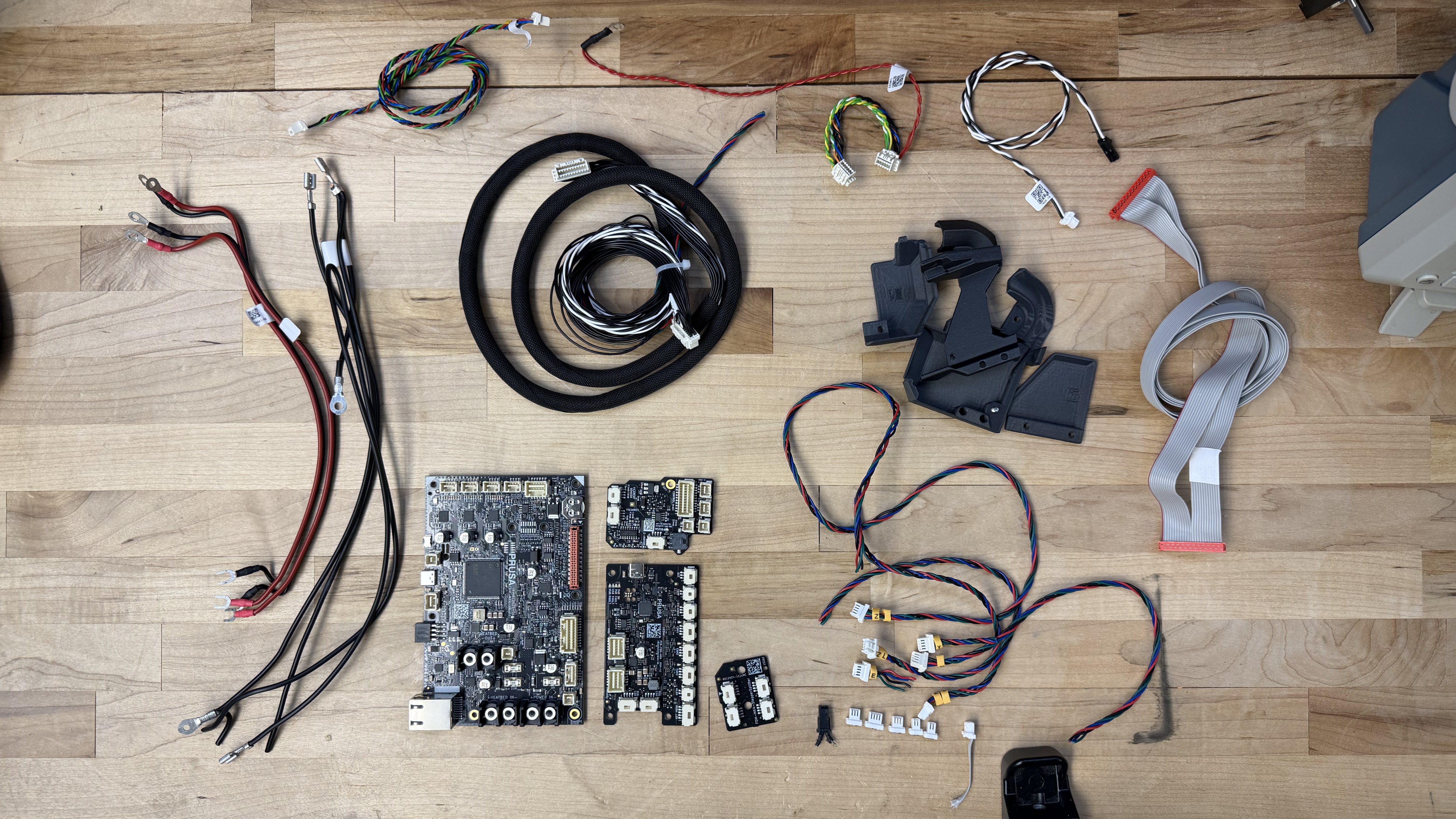
Total board area is about equal.
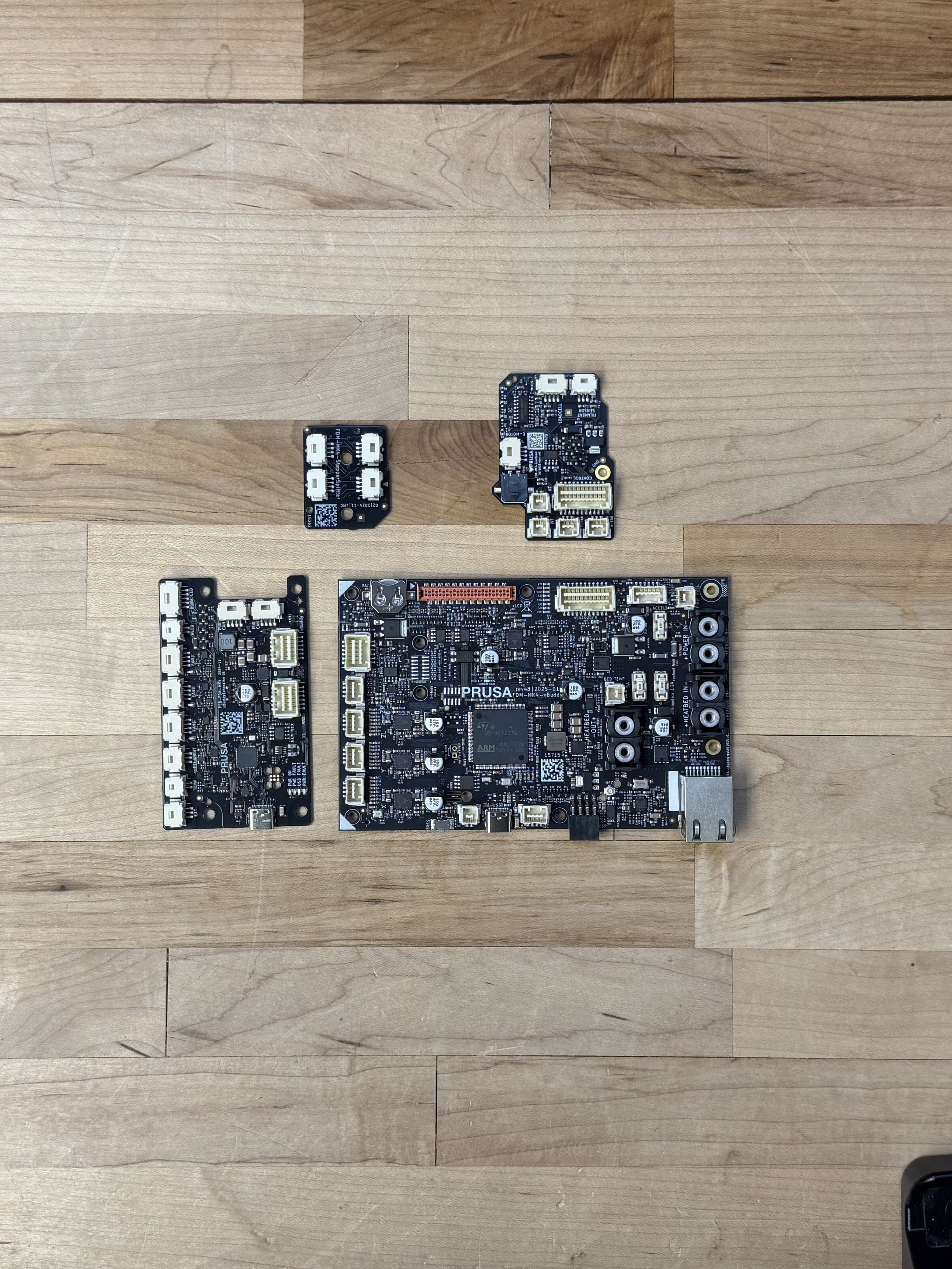
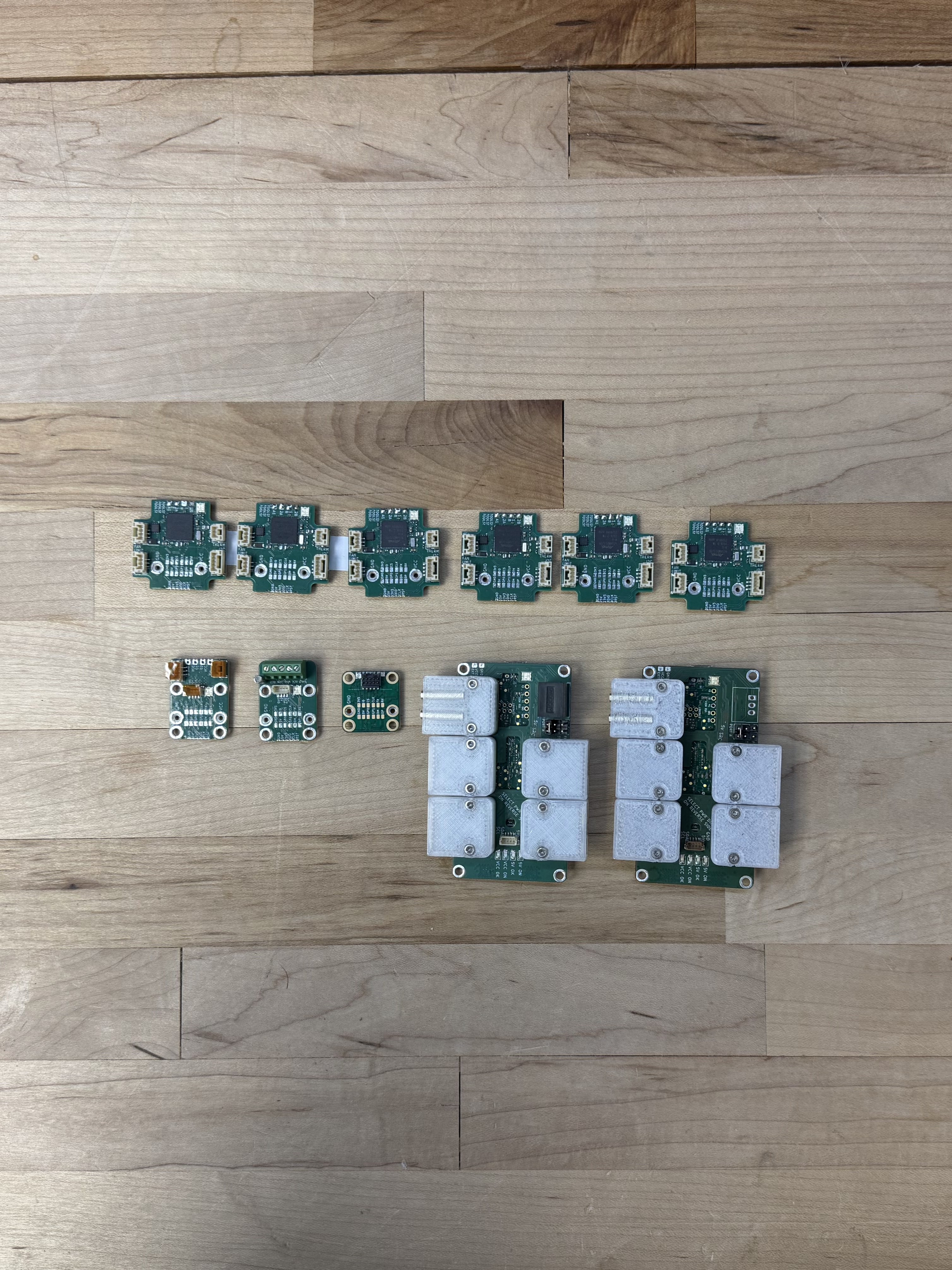
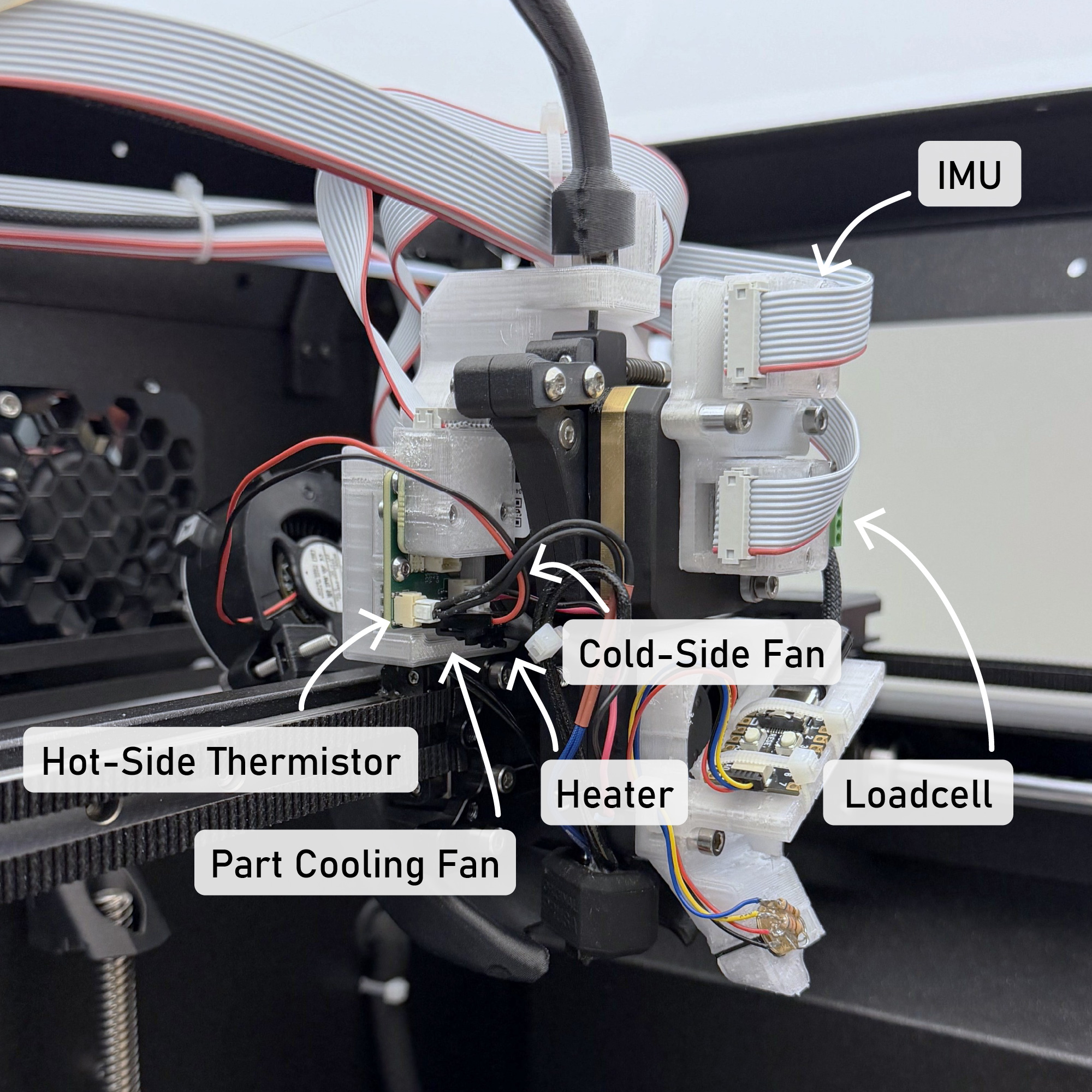
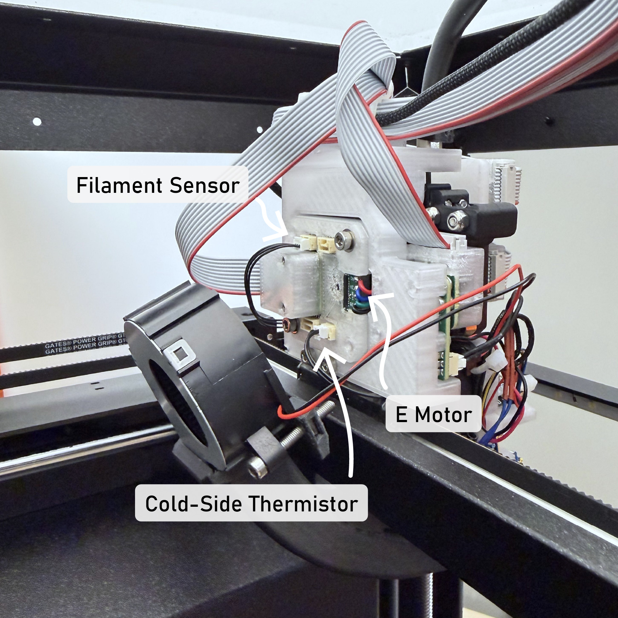
Everything removed from the Prusa. Modular systems simply chassis wiring.
This (plus motor encoders) is the relatively thin interface that the controllers use to sense and control the machine.
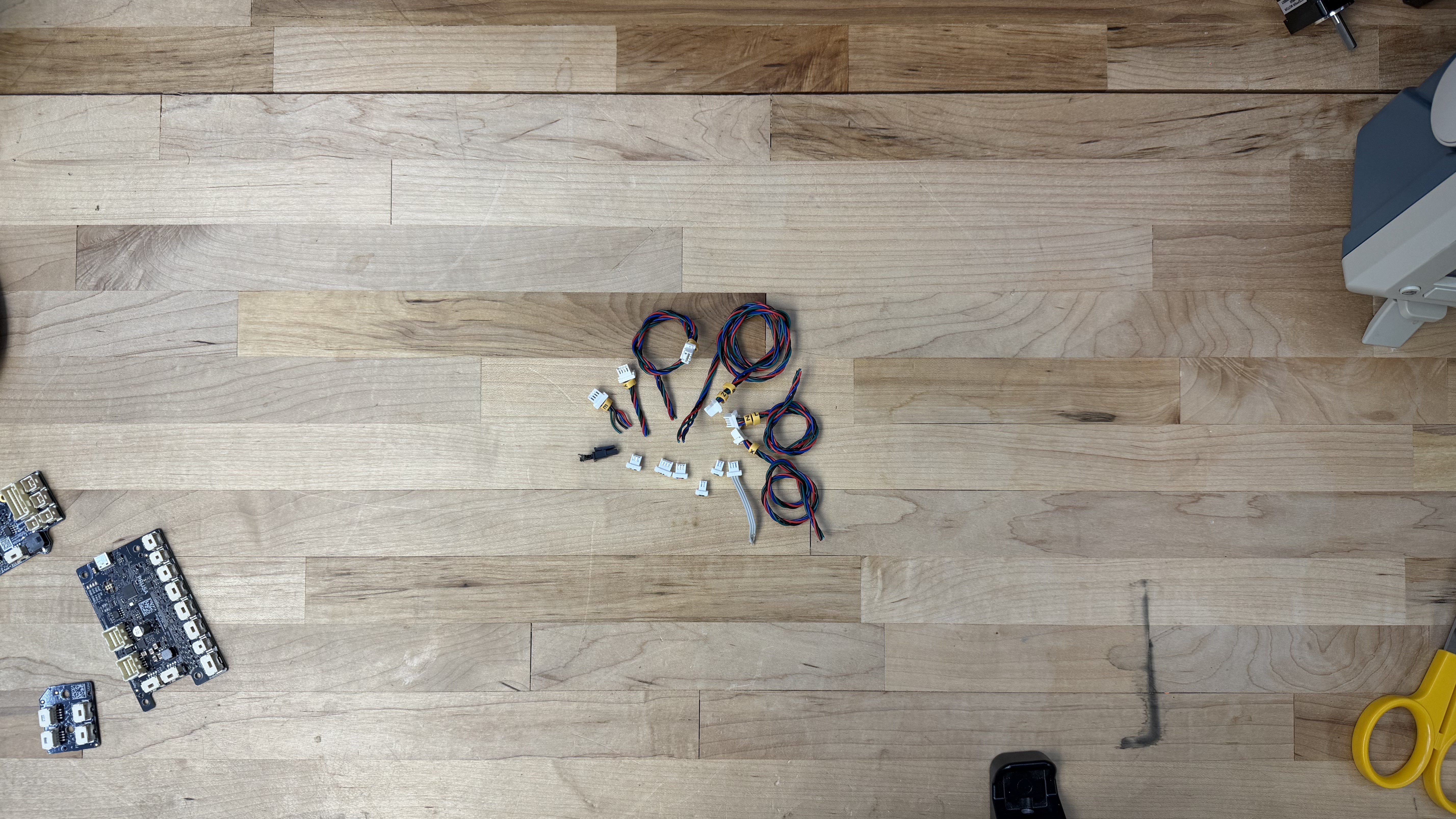
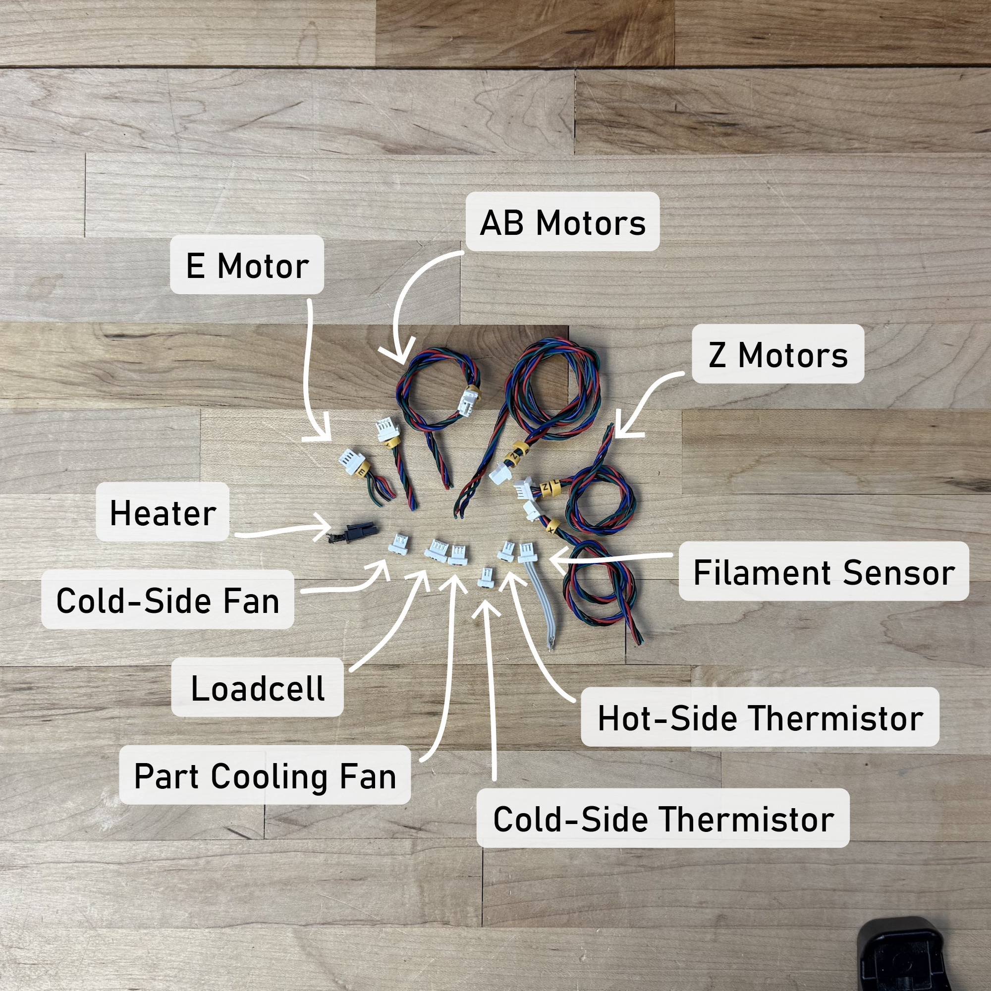
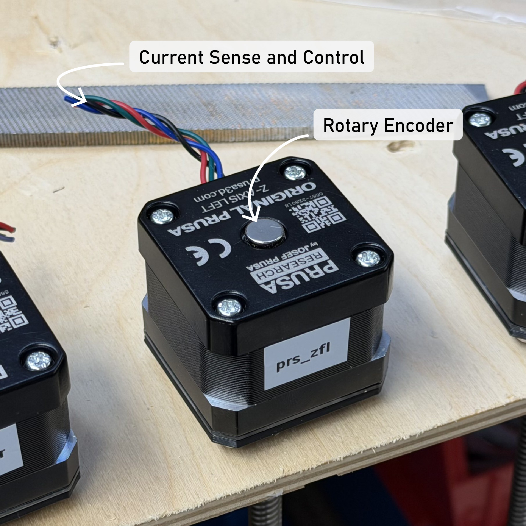
Modules help us re-deploy hardware in multiple contexts, but how do we communicate and coordinate their actions?
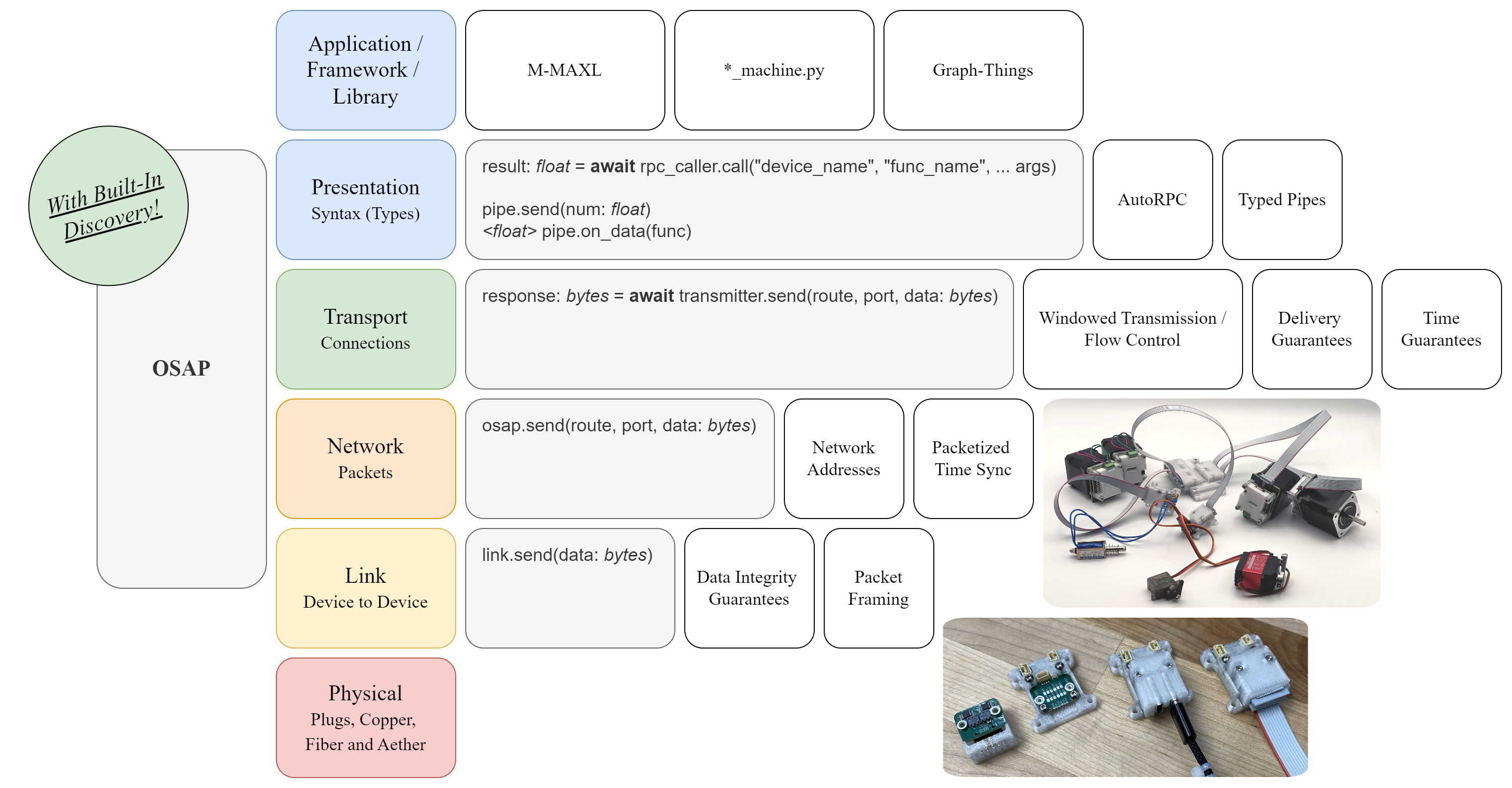
Messages are source routed, meaning there is no stateful network configuration to manage.
Hubs are a design convenience, but not required by the protocol. Any device can pass messages across multiple ports.
Python scripts and device firmwares are peers in the network, and message-passing is link agnostic.
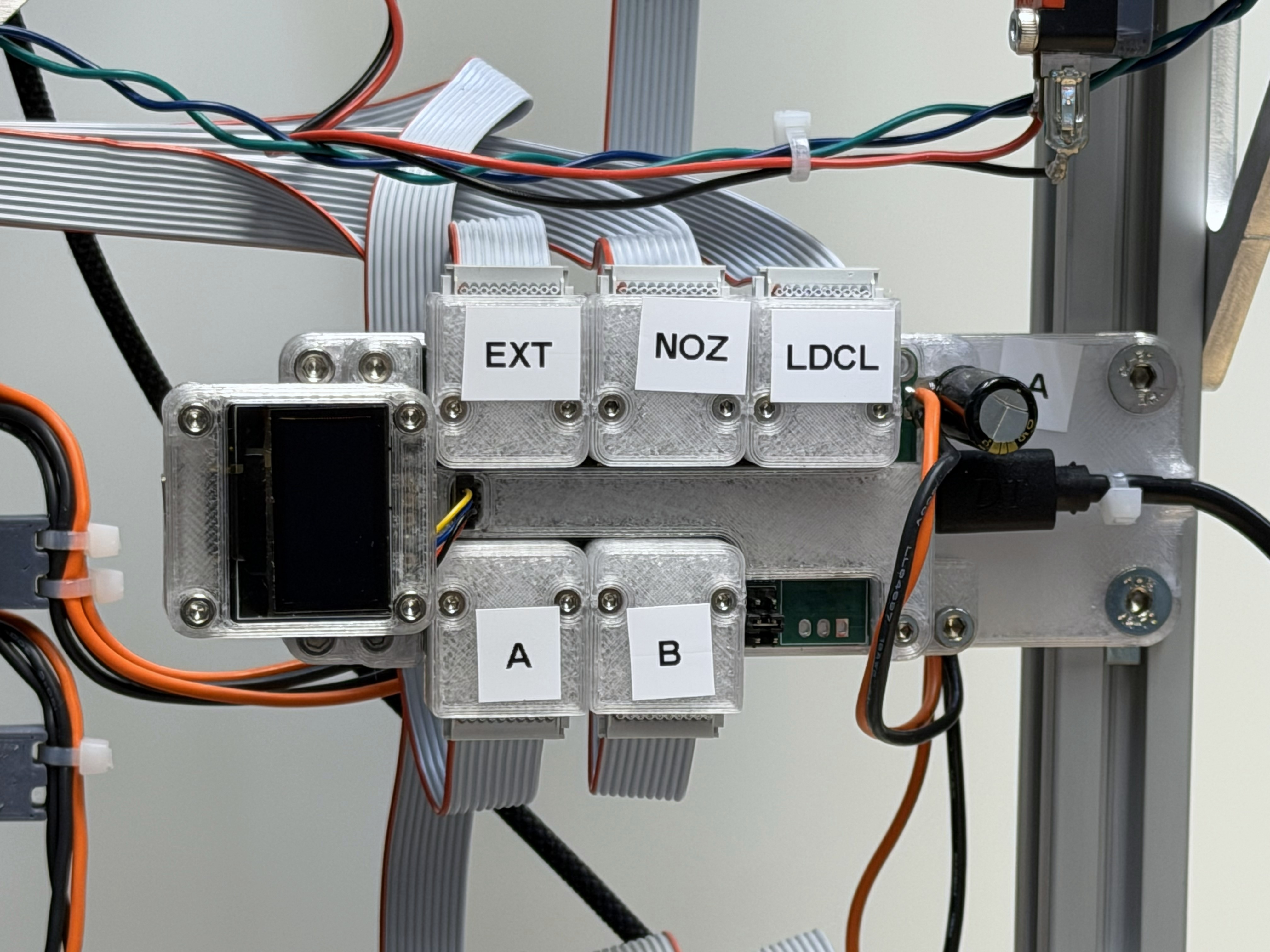
Message-passing hub (one of two used) in the RheoPrinter.
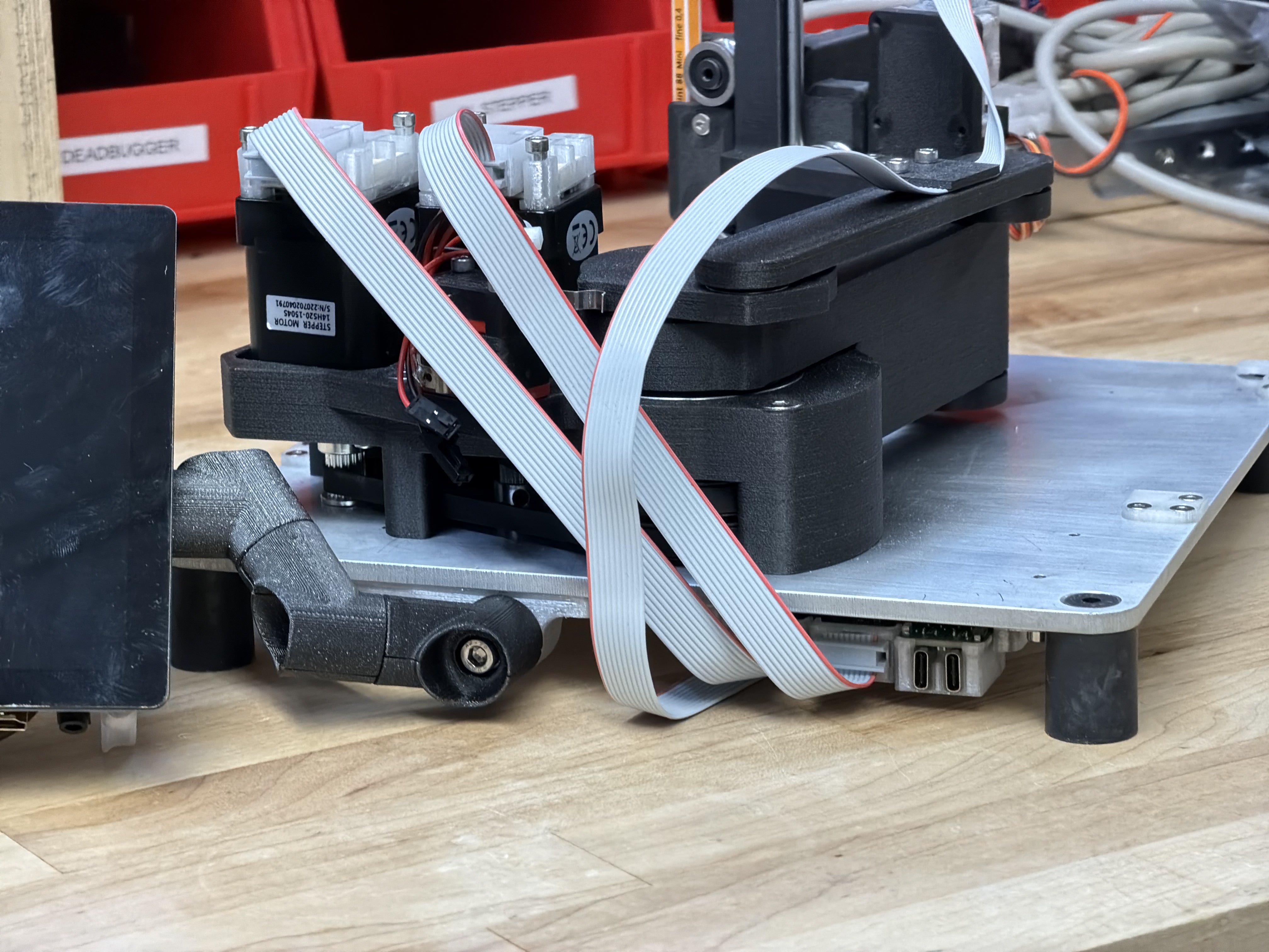
Message-passing hub in the Little Guy.
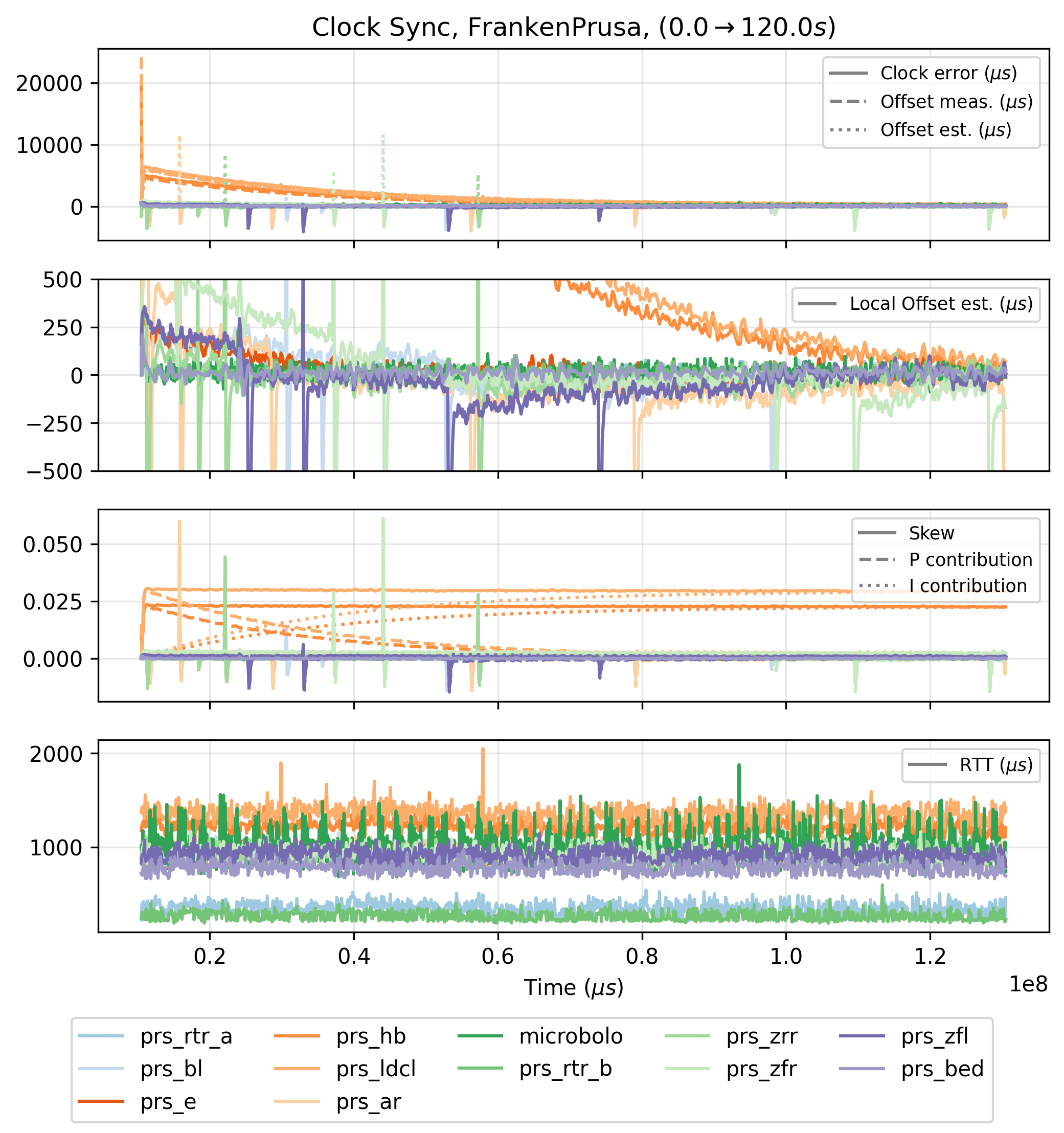
OSAP synchronizes device clocks continuously, providing a basis for coordinated motion control and sensing.
In the printer, clocks typically adjust to within $500\mu\mathrm{s}$ with one another after $60s$ and within $250\mu\mathrm{s}$ after $100s$ - and get better over time.
To avoid waiting for sync every time we start machines, clock skews can be stored and restored at launch.
How is motion synchronized across actuators?
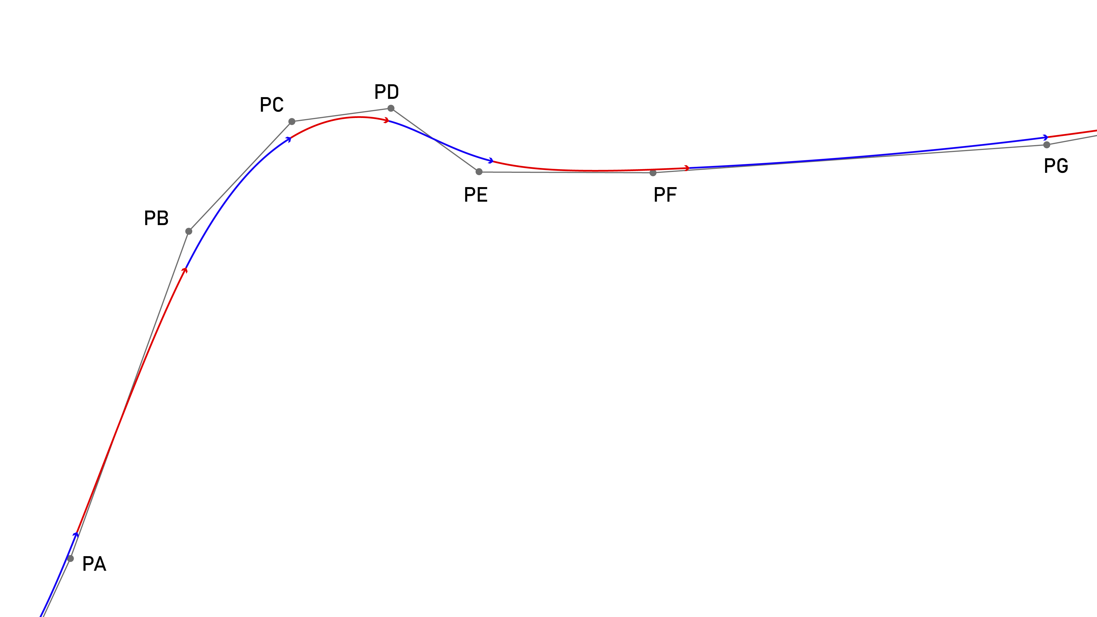
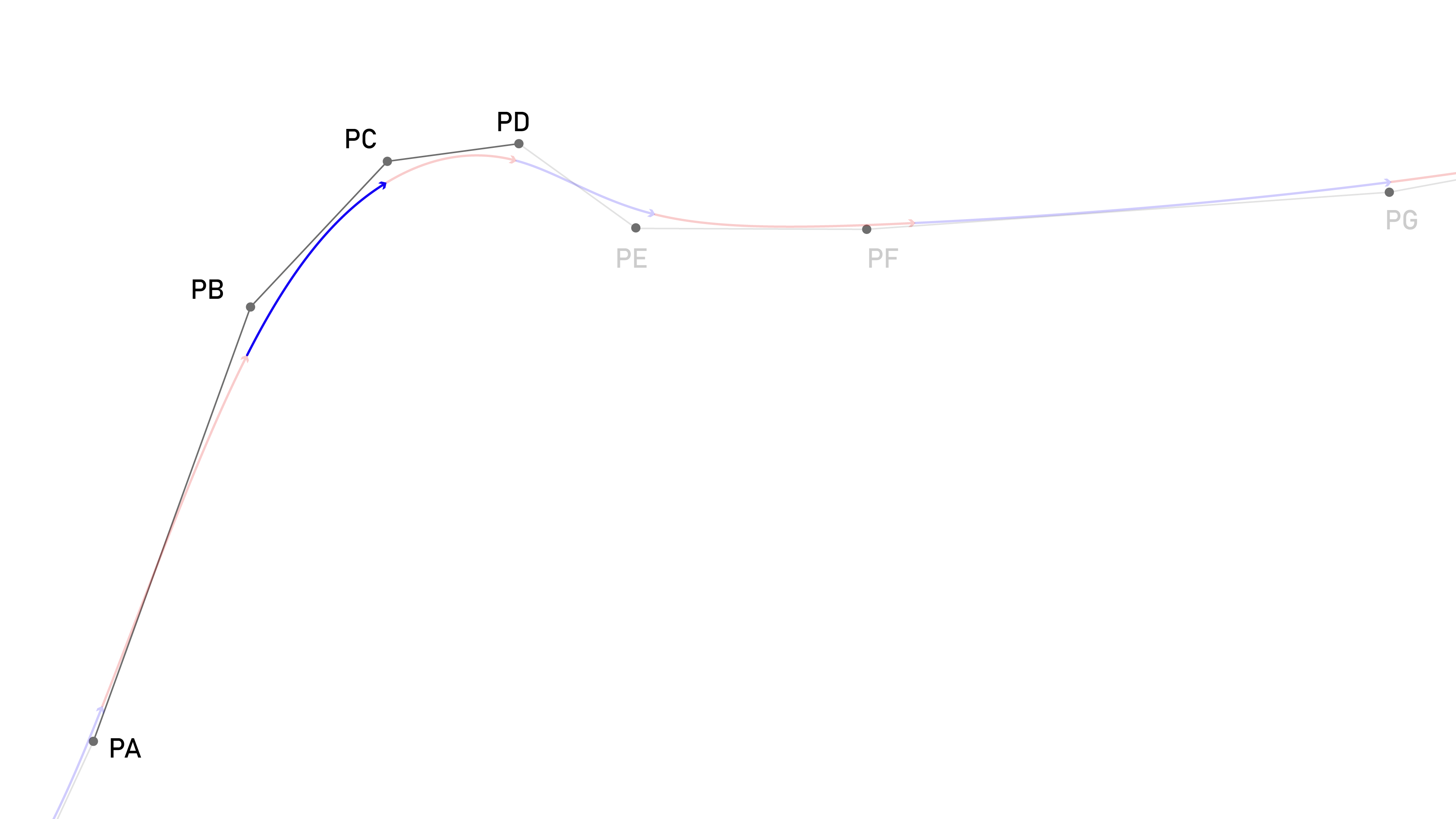
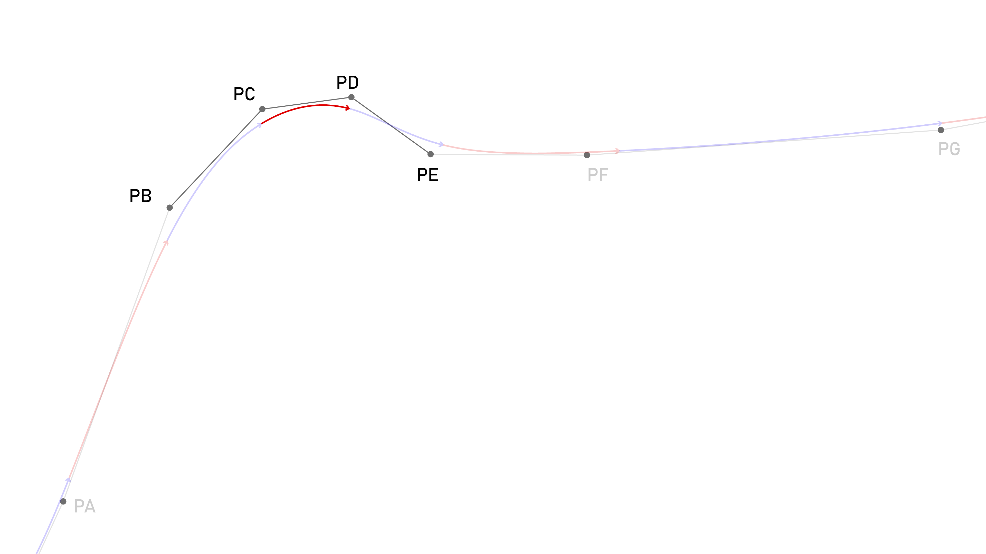
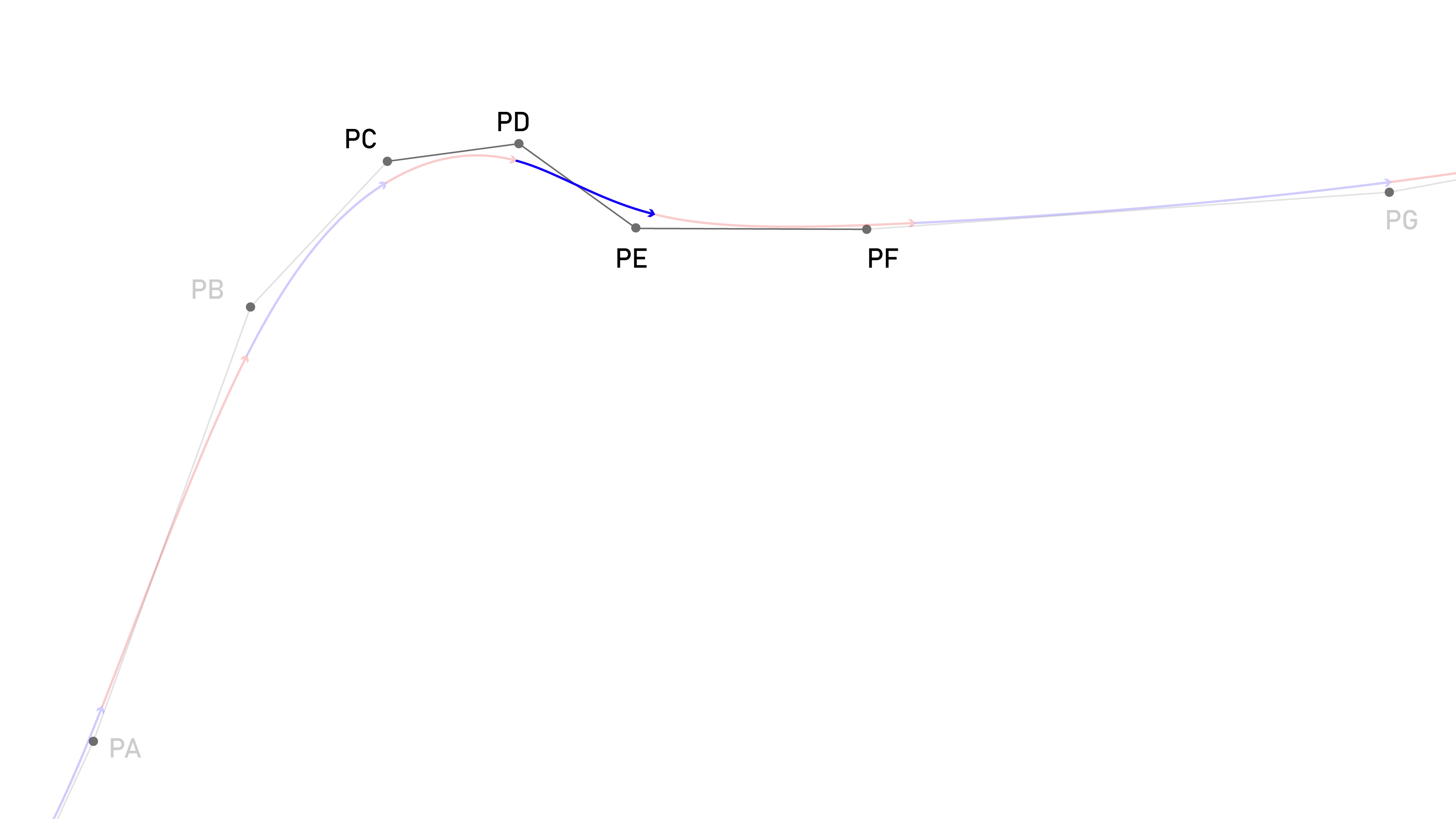
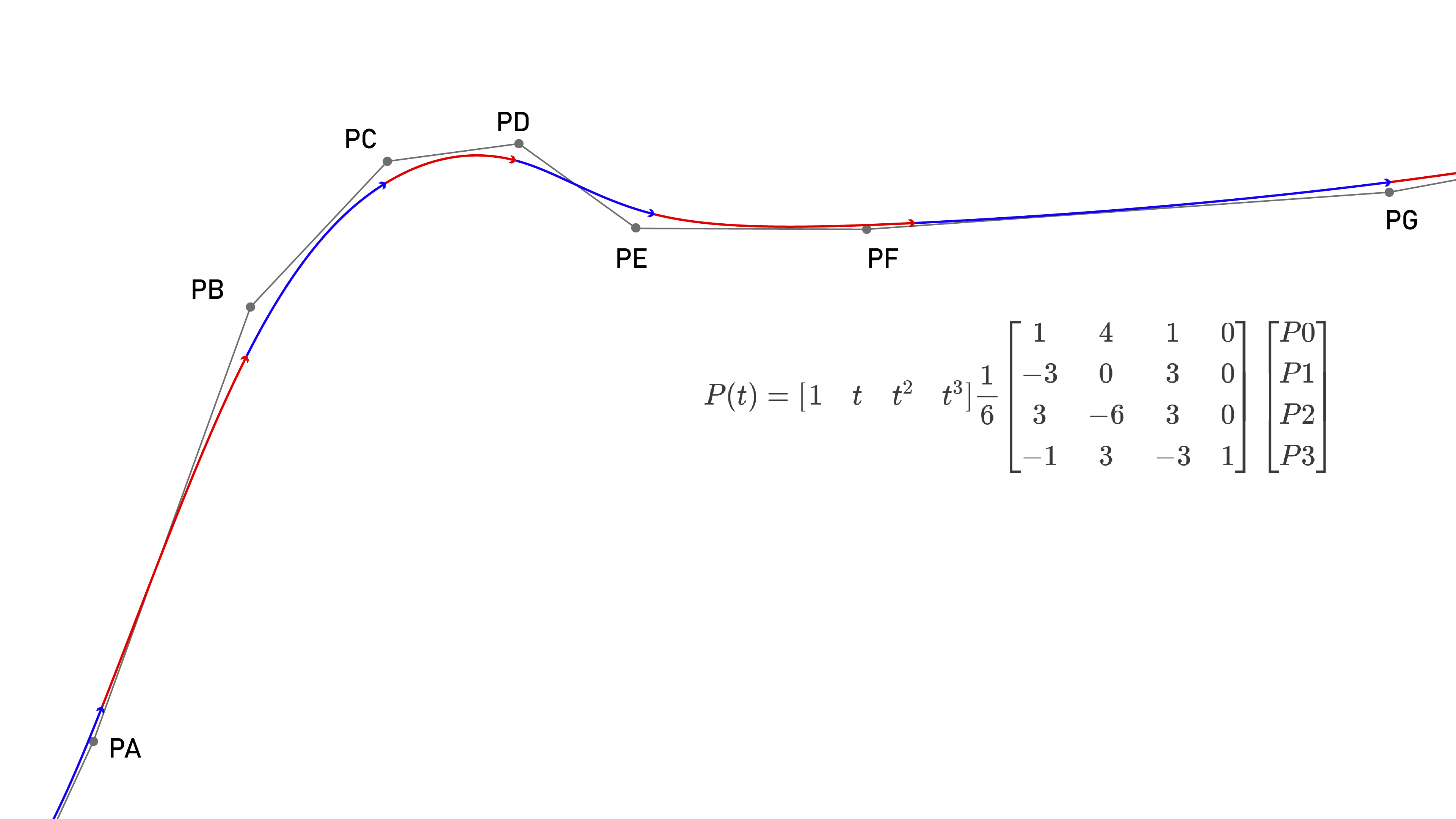
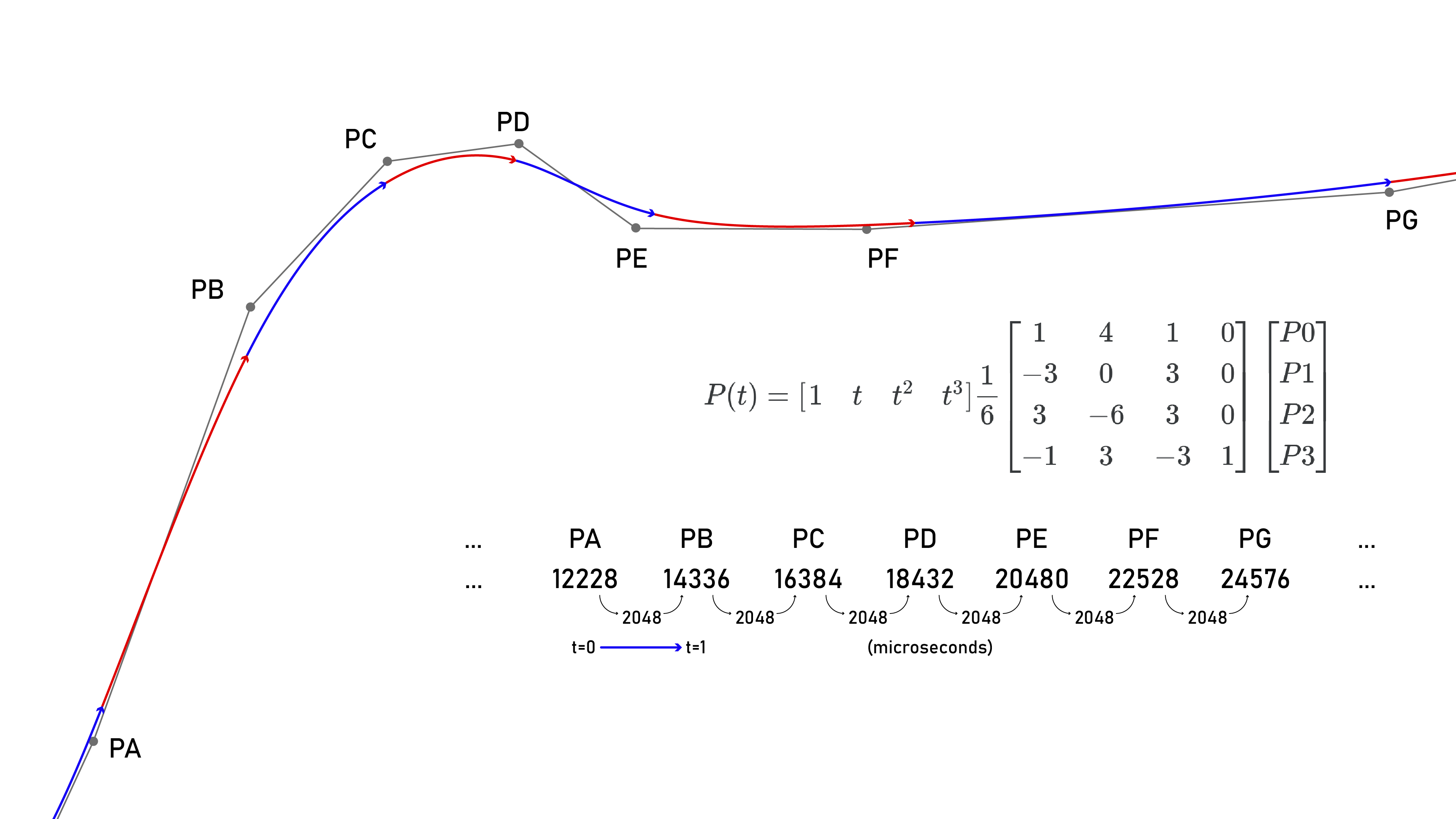
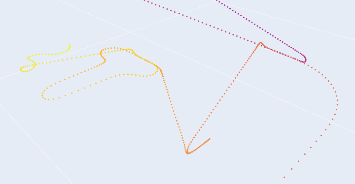
Fixed-interval basis spline segmentation means that network loads are deterministic when we run machines.
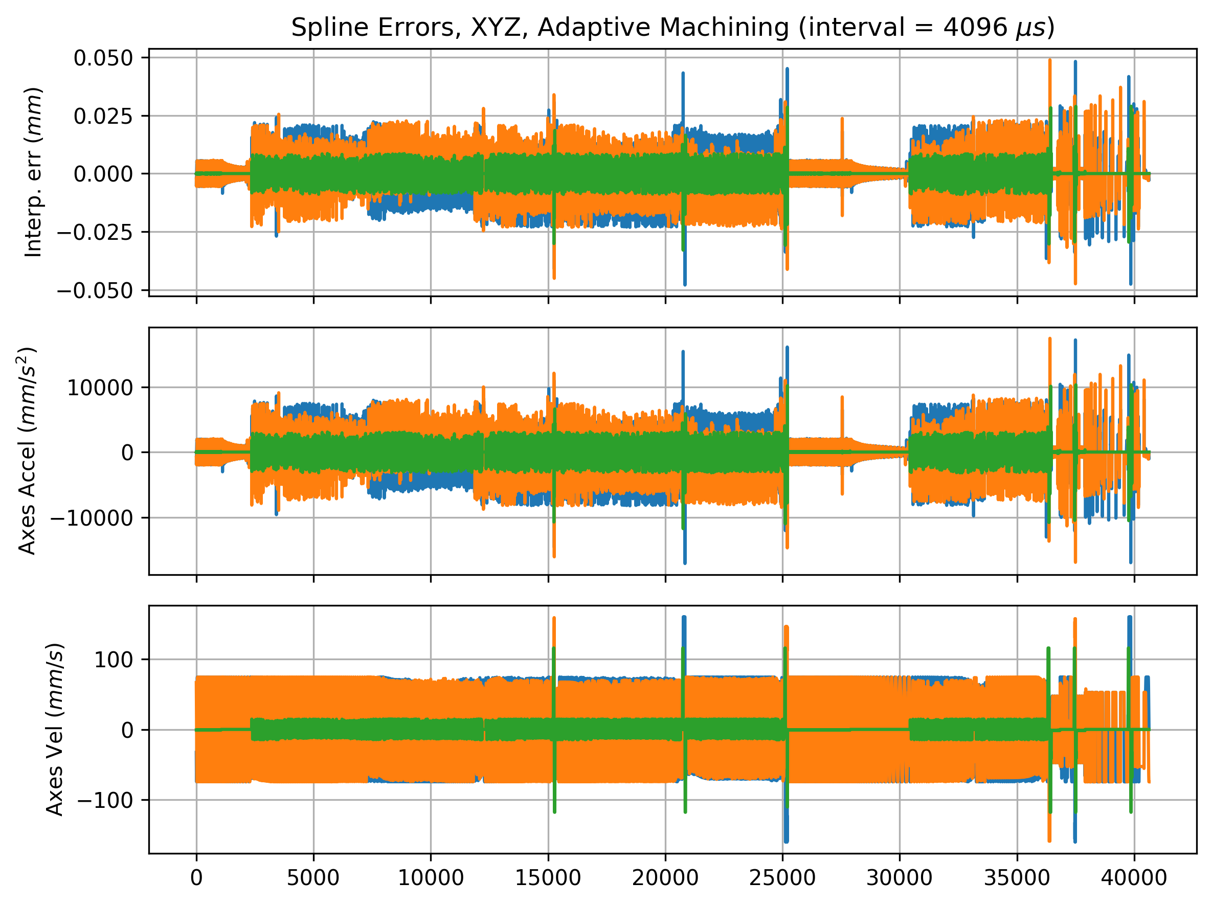
With slow intervals $(4.096ms)$ and high acceleration $(15 000mm/s^2)$ interpolation errors can reach $50\mu m.$
How do we describe machine controllers? Reconfigure them?
Firmwares contain function implementations.
// in hbridge firmware
float readAvailableVCC(void){
	const float r1 = 10000.0F;
	const float r2 = 470.0F;
	// it's this oddball, no-init ADC stuff,
	// teensy is 10-bits basically, y'all
	uint16_t val = analogRead(PIN_SENSE_VCC);
	// convert to voltage,
	float vout = (float)(val) * (3.3F / 1024.0F);
	// that's at 10k - sense - 470r - gnd,
	// vout = (vcc x r2) / (r1 + r2)
	// (vout * (r1 + r2)) / r2 = vcc
	float vcc = (vout * (r1 + r2)) / r2;
	return vcc;
}

// one line to generate an interface
BUILD_RPC(readAvailableVCC, "", "");
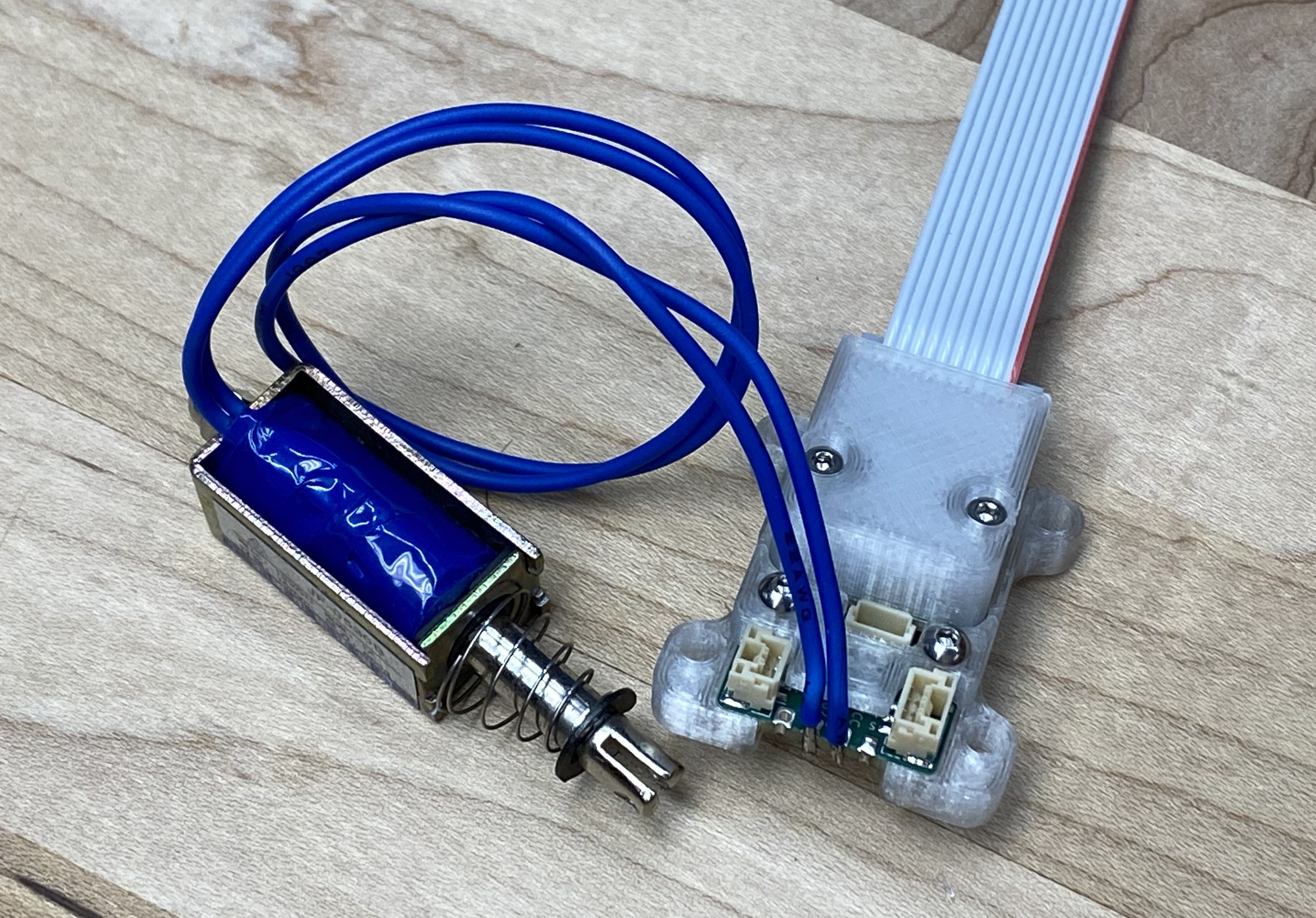
We can access those from other contexts
via proxy classes.
# auto-generated proxy,
class HBridgeProxy:
	# ...
	async def read_available_vcc(self) -> float:
		result = await self._read_available_vcc_rpc.call()
		return cast(float, result)
	# ...
These interfaces are generated automatically, using information
provided by the firmware.
We can use those interfaces to author, debug and modify high-level logic without mucking
about in hardware.
# discover all devices
system_map = await osap.netrunner.update_map()

# build a proxy, check existence
hbridge = HbridgeSamd21DuallyProxy(osap, "hbridge_dually")
try:
	await hbridge.begin()
except NameError:
	print("no hbridge found, check connections...")

print("... request voltage")
await hbridge.set_pd_request_voltage(15)

print("... await voltage")
while True:
	vcc_avail = await hbridge.read_available_vcc()
	print(F"avail: ${vcc_avail:.2f}")
	if vcc_avail > 14.0:
		break

print("pulse...")
for _ in range(100):
	print("...")
	await hbridge.pulse_bridge(2.0, 1000)
	await asyncio.sleep(1.75)
	await hbridge.pulse_bridge(-1.0, 50)
	await asyncio.sleep(1)

print("... done!")
Automatic generation of software interfaces: single-source-of-truth, self-describing modular devices
for distributed systems.
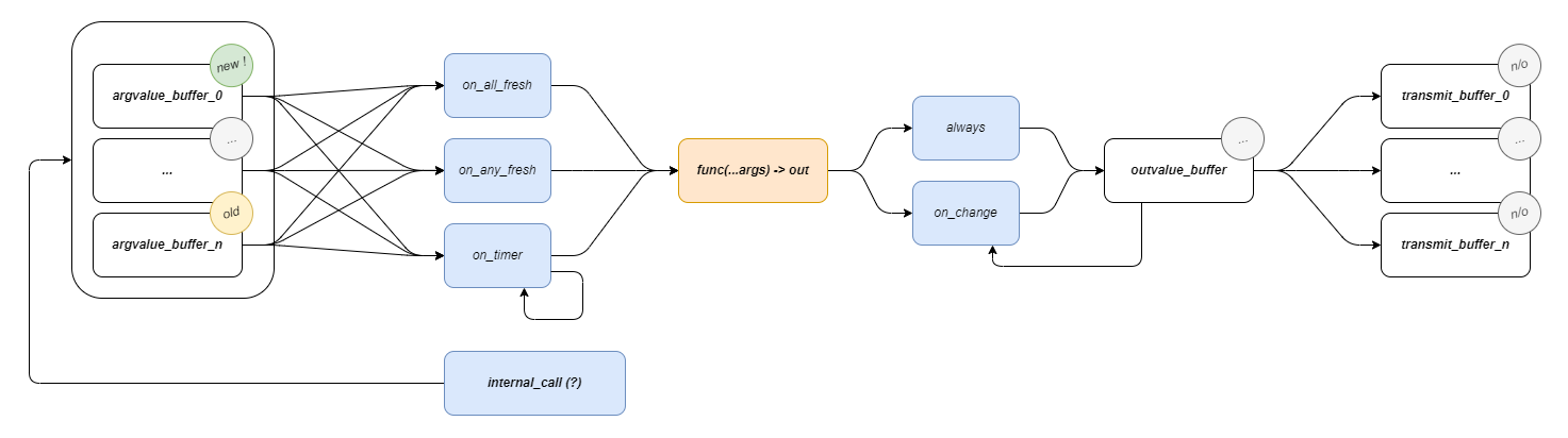
Functions are exposed as graph interfaces as well as RPCs.
# MAXL clock to the solver,
await manager.connect(machine.timer.clock_out, solver.on_new_pt)
# and solver -> dofs,
await manager.connect(solver.on_new_pt, machine.dof_x.on_new_pt, "0, 1", "0, 1")
await manager.connect(solver.on_new_pt, machine.dof_y.on_new_pt, "0, 2", "0, 1")
await manager.connect(solver.on_new_pt, machine.dof_z.on_new_pt, "0, 3", "0, 1")
await manager.connect(solver.on_new_pt, machine.dof_e.on_new_pt, "0, 4", "0, 1")
They can be connected together algorithmically.
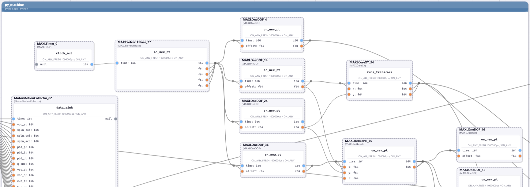
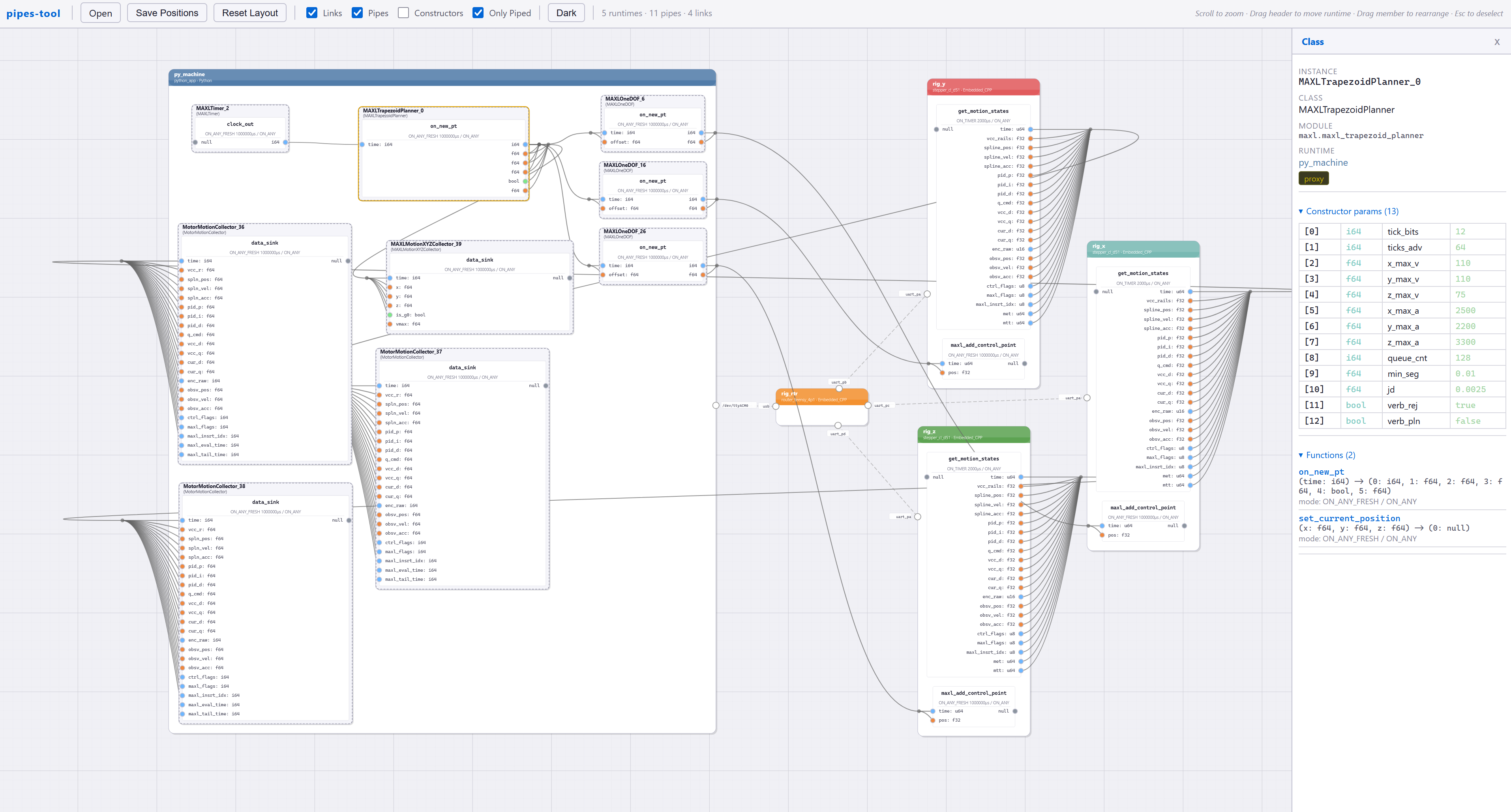
Controller for the milling machine; a mixture of python (boundary with blue top bar, left) and embedded devices (right).
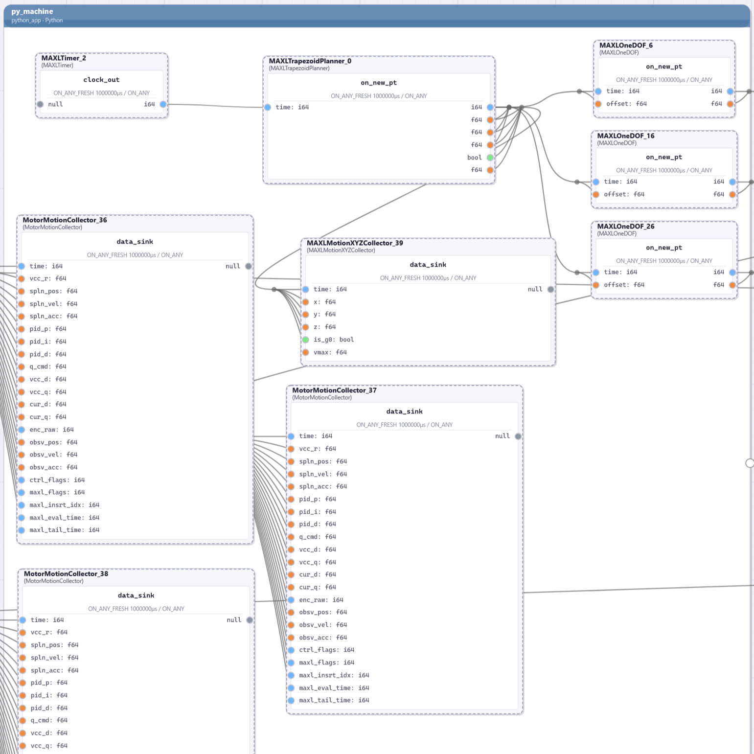
PIPES / MAXL graph for the milling machine, where the trapezoid solver is deployed.
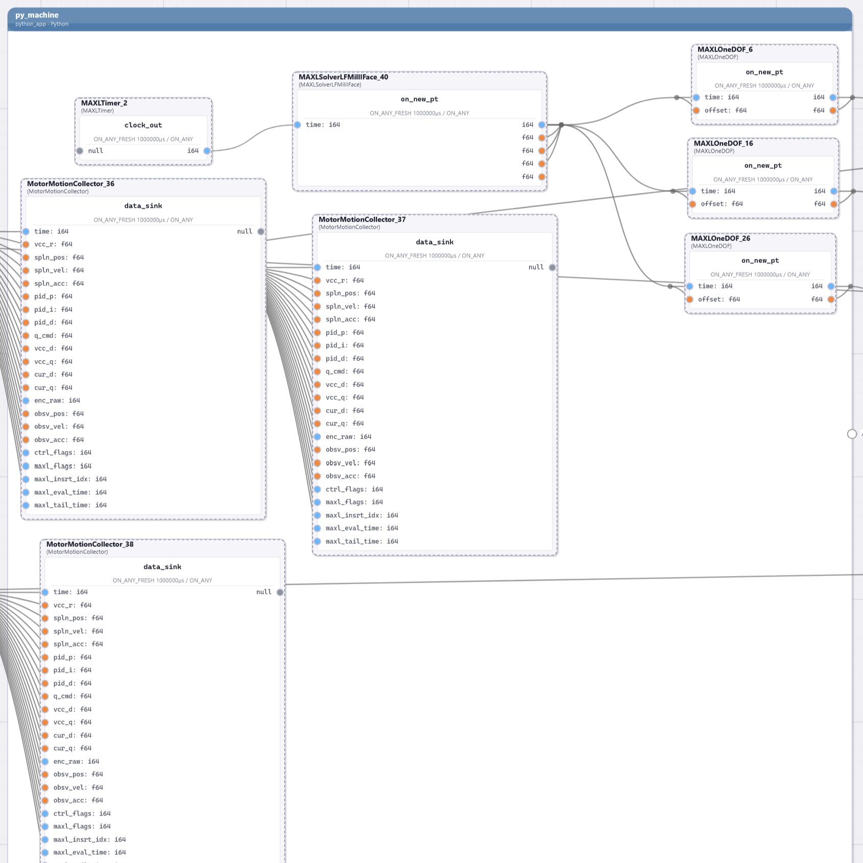
PIPES / MAXL graph for the milling machine, where the optimization-based solver is deployed.
# SETUP the Runtime and Hardware:
osap, manager = await network_tools_setup()

# we can define virtual machines,
machine = Mill(osap, manager,
	MillSetupConfig(
		use_motion_chirp=True,
		use_x= True if test=="chirp_x" else False,
		use_y= True if test=="chirp_y" else False,
		use_z= True if test=="chirp_z" else False,
	)
)

# this step checks that hardware in the machine definition
# is actually connected...
routers, devices = await machine.setup_devices()

# SETUP the Chirp Test
# make a data store,
collector_x = MotorMotionCollector(samps_collect_max)

# connect *most* of the machine controller,
await machine.setup_kinematics()

# connect the x motor's data output to the collector's input:
mot_x = machine.require_x_motor()
await manager.connect(mot_x._get_motion_states_proxy, collector_x.data_sink)

# and then set the PIPES function to run on a timer,
await mot_x._get_motion_states_proxy.set_input_mode('timer', hz_motor_up)
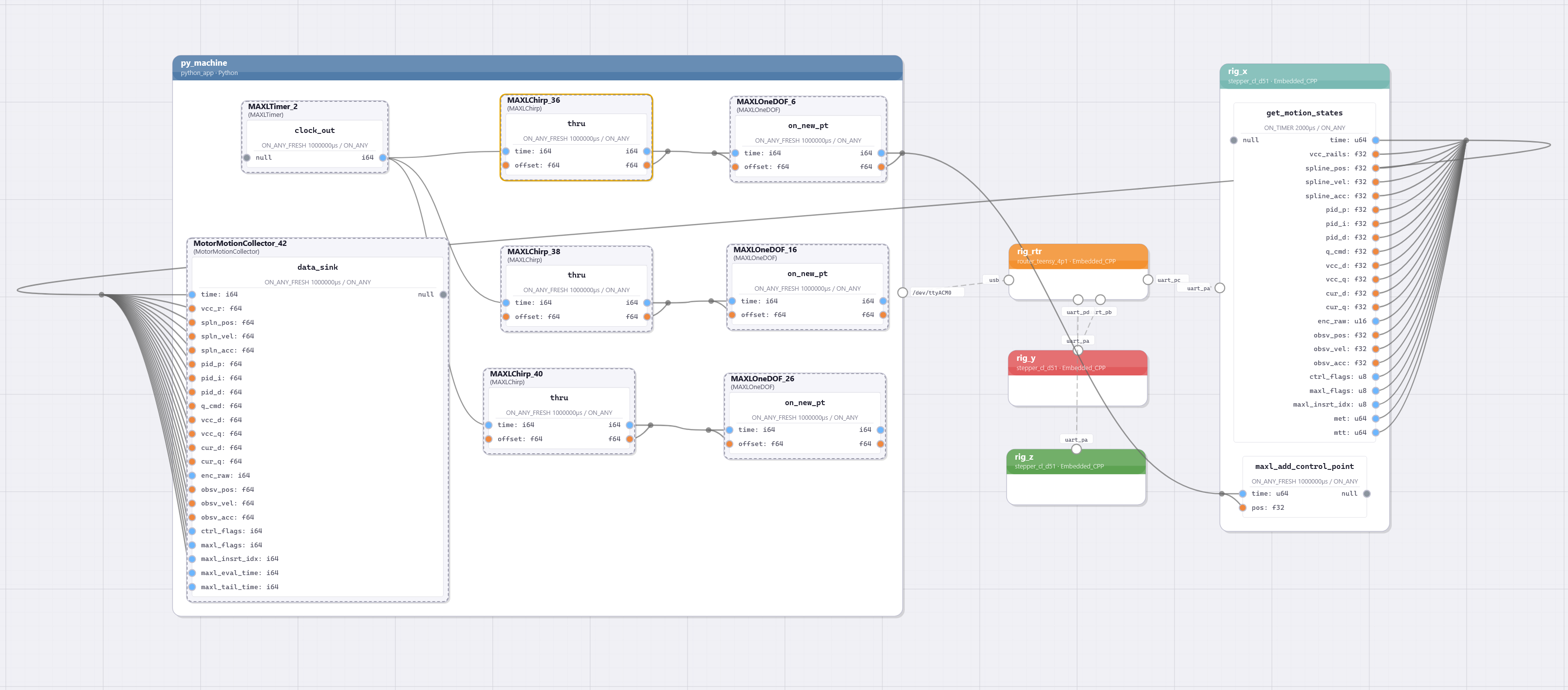
At left is the `setup` code: using OSAP and PIPES to instantiate the machine, confirm that the correct hardware is
connected, and make connections between relevant motion control blocks.
Below, using Remote Procedure Calls to task the machine.
# RUN:
# power it all up,
await machine.ready_motion()

# run a test:
# send a few trapezoid tests
for _ in range(4):
	machine.dof_x.goto_pos(25)
	await machine.dof_x._wait()

	machine.dof_x.goto_pos(-25)
	await machine.dof_x._wait()

# return to (0)
machine.dof_x.goto_pos(0)
await machine.dof_x._wait()

# send a chirp signal,
chirp_x, chirp_y, chirp_z = machine.require_chirp_inputs()
# send one-such chirp,
chirp_x.do_chirp(duration=30, f0=0.5, f1=3.0, amplitude=30.0, tukey=0.85)
while chirp_x._is_chirping():
	await asyncio.sleep(0.1)

# end test, post data:
data = {
	# motor params, traces,
	"test_name": test,
	"run_start_time": run_start_time,
	# motion,
	"mot_params_x": asdict(mot_x_params),
	"motx": collector_x._get_dict(),
}
With re-useable machine modules, we can build new controllers in days rather than weeks or months.
Flexible software lets us develop multiple workflows on the same hardware:
for model fitting, or model use, or swapping controllers entirely in software.
Model-based controllers could help to retrofit equipment that we don't have much data on.
OK.