2 Systems Integration for Modular Machine Control
Up and Running
2.1 Introduction
So, GCode splits our computational representation of machines across the “realtime boundary” (1.4.2). This means that overall machine operation is defined at many layers: by configurations and their associated algorithms in CAM tools, GCode interpreters, and lower level controllers like motor drivers. Those are normally set up by hand1 and the underlying algorithms are often hidden and stateful, making it difficult to ascertain what will happen when we input new machine instructions or make changes to isolated components; this is the black boxing that I discussed at the very start of the thesis in Section 1.3.2 and 1.3.3.
On the other hand, if we can connect across this boundary we stand to improve machine control overall; connecting real physical constraints to planning algorithms, sourcing configurations from hardware rather than aligning them manually, and integrating machine controllers directly into new workflows to enable more interactive operation of hardware and tighter couplings between motion and process controllers.
Taking a cue from software design, we also want to build machine systems from a reusable set of components across hardware (motor drivers, sensors etc.) and software (motion planners and modelling routines). Doing so lets us re-use modules across projects to quickly compose new systems from the parts bin rather than re-engineering circuits, drivers, and code.
So, the focus of this chapter is to develop a set of systems integration tools that “span” the realtime gap, connecting big and small modules in a distributed runtime and developing a programming model that can configure and coordinate global operation of devices within that runtime. This will focus first on networking technologies, and then on the development of a programming model to suit.
2.1.1 Machine Building Needs Flexible Network Architectures
In practice machine-scale modular hardware systems are deployed on a heterogeneity of different network links and transport layers [1] whereas the internet is dominated by only a few (TCP, Ethernet, WiFi, etc). This is true for the same reason that many different types of machines exist: the physical world is itself heterogeneous. Sometimes we want networks to be cheap, sometimes we want them to be extremely performant, sometimes noise immunity is critical, and other times it is not; this leads to a proliferation of different networking technologies. Because embedded devices are low on computing power, building clean interfaces between network layers is not top-of-mind for automation engineers2 and because machines tend not to be required to integrate within larger networks there is little industrial pressure to develop interoperability across network architectures.3
The Open Systems Interconnect model (OSI [2]) developed by the international organization for standards (ISO) is meant to separate network layers from application-level concerns so that we could plug almost any device into almost any system. This follows the end-to-end principle [3], which proposes that systems be designed such that modifications to their ends (applications) not require updates or modifications to systems architectures themselves. The heterogeneity of machine control networks means that we really need the OSI model to work for automation perhaps more than we do for the internet. However, the OSI model is only “loosely” followed by most modern networks [4] and industrial networks in particular tend to collapse layers. CAN bus [5] (common in automobiles and simpler robotic systems) is perhaps the best example: we can only run CAN-type application layers on CAN busses, e.g. CANopen [6] and J1939 [7]. EtherCAT [8] [9] collapses the OSI layers for routing and transport: connecting devices on an EtherCAT network to nonlocal applications requires special tunnelling protocols. Time synchronization of one EtherCAT network to global time via the internet’s precision time protocol (PTP, [10]) requires a special bridge.
This divergence in systems is not due to a simple lack of better standards; network performance constrains realtime control of hardware in important ways as I will discuss in more detail in 2.2.2.1; the through line is that networks for control should be performant and also deterministic. In fact EtherCAT’s collapse of intermediate layers is done explicitly to remove overhead in those layers and thus increase performance, and CAN based networks are constrained in the application layer because CAN packet structures and application semantics are themselves combined in order to reduce packet overhead.
It is easy to imagine simply improving network systems’ performance to the point where we could alleviate those constraints on architectures themselves (making room for network abstractions and layers), but the requirement for determinism bleeds more broadly into systems design. For example to build reliable networked controllers, accepting arbitrary network traffic from outside is often unwise: we would not want to expose those systems to DDoS4 attacks or (for a more reasonable scenario) to be modified to the point where bandwidth consumed by new modifications saps the performance of previously reliable networks.
So, try as we may it is not really possible to separate the design of our networked applications from the design of networks themselves, or the design of the computing systems that run those applications. This is the scheduling problem, where we must take some set of tasks (an application) and run those in a constrained amount of time (available on network links in terms of bandwidth limits, and on computing devices in terms of clock cycles).5 The main difference between purely informatic networks (like most of the internet) and networks that control machines and robots is that the former has much more relaxed time constraints, whereas in the latter failures to pass messages in time can make for unsafe behaviour. There are advanced algorithmic approaches to scheduling that provide good solutions6 to the challenge, but none can completely guarantee optimal performance because scheduling is NP-Hard. Articulating network behaviour and programs themselves completely is also difficult, so in practice systems are often designed by hand against worst-case analysis [11] and then tested for safety — modifications to these systems are then difficult to make without re-assessing their schedules.
The scheduling problem itself is well outside the scope of this thesis, but it is an important consideration as we design networks. Comprehension of the networked systems over which distributed programs are run is a critical step in solving the scheduling program either by hand or algorithmically; we are also motivated to build systems that have built-in mechanisms for feedback and measurement.
One final note on our motivations with regards to networking systems: embedded networks can fall under the purview of professionals whose main practice is not in information technology itself. The assembly of the internet (and its integration within businesses, homes etc.) is mostly carried out by network professionals, whereas machine design firms, factorys, or open source machine developers are less likely to be as completely versed in the nuances of network design. For this reason again we are motivated to make network systems that require minimal manual configuration and that provide some degree of flexibility and inspectability.
2.1.2 Machine Building Needs Flexible Software Architectures
Connecting devices over networks is not enough, we also need a programming model with which to use them.
While partitioning machine systems across the realtime boundary makes excellent sense from a reliability and determinism point of view, machine controllers are in practice a smaller part of much larger and more complex workflows; managing multiple layers of configuration and statefulness can end up limiting the development of those workflows. For example in the introduction I discussed how this partitioning prevents us from connecting high-level tasks like CAM from low-level constraints that can be seen by controllers; this makes it difficult to articulate machine control overall as a constrained optimization task or otherwise apply modern, intelligent controls strategies. In one of the background sections here (2.2.4.7) I show some examples of other research where machines are integrated into new workflows via GCode wrappers; software objects that expose machine functionality with an API but use GCode “under the hood” to control hardware. This approach is itself invaluable in the first pass, but then tasks like extracting real machine state, modifying motion parameters, configuring kinematics, or synchronizing control with motion trajectories becomes an issue. I make note of similar limits for state-of-the-art modelling of motion control systems themselves in Section 4.2.8 and I survey other improvements to controller partitioning in 2.2.4 and discuss difficulties in extending and reconfiguring GCode interpreters themselves in Section 2.2.1.
However, we cannot simply collapse the realtime boundary and e.g. use one monolithic program to operate the whole controller, so the architectural challenge is this: having partitioned our control systems, what kind of programming model can represent algorithms that span those partitions.
A machine programming model needs to work for two basic tasks: configuration and operation, aka to get our hardware up and running. The first means making sense of which devices are in the system and connecting them to one another according to some control logic. This includes configuration of software modules throughout the system, but we will want to be able to do this without re-compiling and flashing firmwares which is time-consuming, cumbersome (especially on large and complex machines), and can easily lead to misalignments between firmware and software configurations. The second is to operate those machines, i.e. task them; deliver trajectories to machines, home and jog them, or describe higher level algorithms that control them etc. — broadly, tell them what to do. While the operation of our machines is partitioned, we would prefer to configure and task them from one place. With the systems I develop here we can develop application-specific scripts that can ascertain and modify the system’s global state and then perform whichever tasks or control steps are required by the application.
Since we have multiple devices in these systems, representing networks and parallelism in the programming model is key; we will also need to develop a common runtime for software within each device such that the execution of local parts of a program is self-similar to operation of parts of the program that run globally.
2.1.3 Chapter Overview
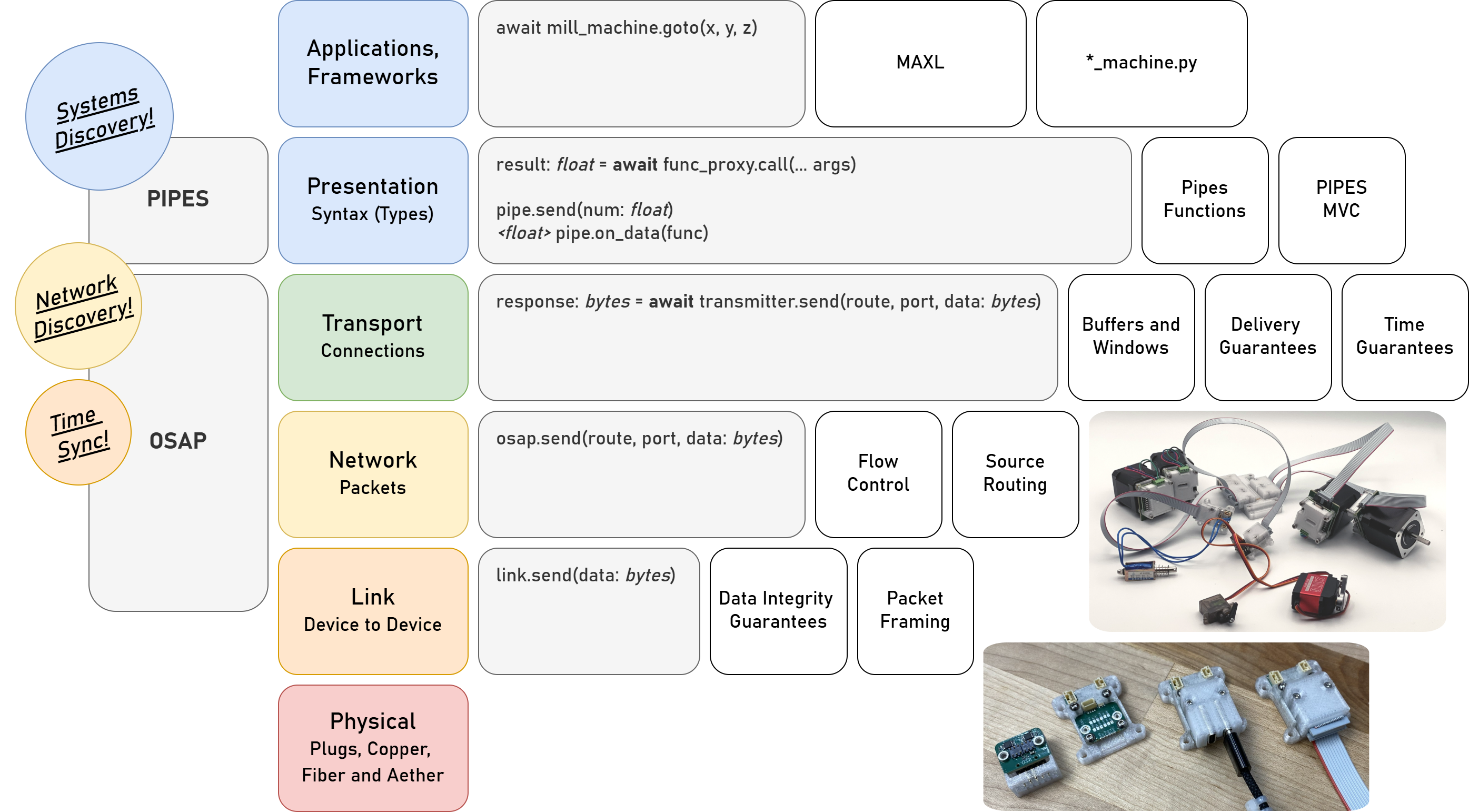
This chapter presents OSAP in 2.3, it is an Open Systems Assembly Protocol and networking runtime that connects hardware and software modules together in one consistent distributed runtime over heterogeneous network links. To build and configure distributed programs in this runtime I build PIPES in 2.4 (for Programming In Piped EcoSystems). It is a programming model that combines dataflow with scripting and includes tools for looking at and configuring partitioned systems, making sense of their global structure. Finally, MAXL (2.5) is set of PIPES modules that express motion control configurations using dataflow so that controllers can be flexibly partitioned. These map to the OSI model for systems interconnect in Figure 2.2.
2.1.3.1 Key Questions and Goals
At its core this chapter is about learning new ways to solve the partitioning problem that I described in Section 1.4, which unpacks into a few more focused questions.
Partitioned systems span two basic representations: networks and the programs that run across them. In the background section on state-of-the-art distributed systems (2.2.3) I show that most of them represent distributed programs using shared data layers that abstract network operation even though understanding network operation is critical to understanding how these systems run. Their integration of truly low-level embedded devices is also limited and indirect even though the operation of those devices is essential for tight control of mechatronic systems. So, how should we formulate an architecture that adds embedded devices to distributed systems as first-class citizens and also extends up into high level computing? Another common pitfall of existing distributed systems is that they require manual alignments across program and network configurations, can we use design patterns from other complex distributed systems like the internet itself and datacenters to resolve this issue, even in much smaller computing environments?
An overarching goal of the thesis is to develop model-based control for machines in order to simplify and improve machine operation and to expose the hidden optimization that I described in Section 1.3.3 so that operators can better understand their hardware and so that planning algorithms and modelling tools can relate more directly to low-level machine states. Doing so involves running substantial parts of the controller in off-the-shelf operating systems where high performance computing is available and systems development is straightforward, but also requires tight integration with low-level embedded controllers. This introduces another series of questions and goals: in this new architecture how should we synchronize motion control outputs written in non-deterministic operating systems with execution across modular hardware, how do we collect data in those systems, and how can we minimize indeterminacy and latency across the networks that span them? Using the same programming model and runtime in operating systems and in embedded devices is likely to limit the capability of high-level compute while introducing overhead in low-level devices, so what is the right balance between complexity and descriptiveness and is there a way to enable simple, low-level operation within devices with complex high-level global configurations?
And what about the programming model itself? Machine operation requires high-level configuration and tasking, but also fast low-level operation, what kind of systems description tool can combine those without introducing undue overhead? Implicit in all of these questions is the goal of building flexible systems that span variable machine kinematics and application, so in each case we have the additional challenge and goal of accomplishing these tasks using modules and learning e.g. how big those modules should be, which subroutines they should contain, how they can be combined across applications and how they should be authored.
In a really compressed framing: the GCode partition lies right in the gap between high-level / operating-systems scale computing and low-level embedded computing. To build better machines we want to connect these layers, so this chapter considers how we should span the gap computationally and contributes new architectural models to do so.
2.1.3.2 Background Overview
The background section (2.2) starts with an overview of the longer arc of machine systems research from my own local environment at the Center for Bits and Atoms (2.2) and then takes a practical look at the problem, showing how off-the-shelf GCode interpreters are partitioned and modified in Section 2.2.1. With that broader context in mind I take a step back and look at relevant research and themes in network organization and network-based control in 2.2.2, and then the same for distributed systems and programming models in 2.2.3, and finally a closer look at machine control specific partitions and architectures in 2.2.4. Each of these aspects of the broader problem are interlinked. Overall the background is about understanding how the partitioning problem from Section 1.4.2 is solved or managed in the state-of-the-art, not just for machine systems but also in broader contexts where excellent design patterns have been developed for similar problems e.g. in the internet itself, and datacenter architectures and massively parallel computing and in other mechatronic systems like spacecraft and robotics.
2.1.3.3 Methods, Contributions and Results
I present this chapter’s architectural contributions in three sections, OSAP (Section 2.3) establishes a common network-oriented runtime within and across distributed devices, routes messages over heterogeneous link layers using a stateless networking scheme, provides synchronization and configuration discovery services and basic performance measurements, and does so within a simplified OSI model. PIPES (Section 2.4) develops a distributed programming model that combines dataflow with scripting to configure and task machine systems using a unified Systems Object Model that combines software and networking. It includes tools for discovery and modification of systems-wide configurations and schemas, and for device API discovery and authorship. MAXL (Section 2.5) develops modular motion control as a series of reusable dataflow blocks for kinematic transforms, offsets, and other reusable control components.
In Section 2.6 I show how these contributions differ and improve on state-of-the-art practice; how they represent of data (2.6.1.1), operation (2.6.1.2), networks (2.6.1.3), and configurations (2.6.1.4) across distributed systems, how they enable tighter integration between model-based controllers and machine networks in a comparison to other state-of-the-art model-based control researchers’ work (2.6.2), and how they add important capabilities to other machine control specific architectures (2.6.3) while simplifying their configurations.
In the start of the results section I summarize key architectural deltas over the state-of-the-art and explain how those enabled other work in this chapter and thesis (2.7.1) which also serves to introduce the results from the chapter. I show how they turn GCodes into code (2.7.3) and that they allow “soft” reconfiguration of hardware for different realtime tasks (2.7.4) and reconfiguration of hardware across different machines (2.7.5) including a litany of kinematics (2.7.5.1). To improve control and feedback, I will show how they expose the hidden velocity optimization simply be moving it from hardware into software (2.7.6) and how they overlay sensor data with controller data for online modelling (2.7.7).
Overall the systems that I develop represent a new combination of design patterns from state-of-the-art practice in a litany of other fields. This includes lightweight networking strategies from early IoT and spaceborne networks, discovery and configuration patterns from datacenters and the web, and composable systems insights from visual dataflow systems. In this thesis they are newly applied to machine control. In doing so we can invent new design patterns for distributed systems that combine high-level and low-level computing while maintaining that low-level devices are first-class citizens, new methods for the operation of machine controllers across the realtime gap in that let us blend non-deterministic but computationally powerful computing with deterministic low-level computing, and new strategies for the rapid reconfiguration of hardware modules and software modules — especially for software-defined motion control using dataflow. We also learn what the key limitations to these architectural deltas are and what types of systems we should focus on developing in the future.
Broadly I would say that the SI tools I develop in this chapter (more so than in other contributions in the thesis) are combinations of other systems and methods. I borrow patterns from datacenter / distributed software systems, from web development, and from other network-based controllers. The main differentiator across these contributions and my own is that these patterns have seldom been applied to machine control: here we have more direct constraints on the time-based performance of these systems and smaller, more heterogeneous computing.
2.2 Background in Systems Integration
Systems integration spans many domains: programming and compute models, API design, networking, etc. A complete discussion of each topic is outside of the scope of this thesis, but I want to cover the relevant constraints and considerations and then look more closely at other researchers’ efforts to improve machine controllers from this perspective: building new ways to configure and program digital fabrication machines and workflows.
So, I will organize this background section from low- to high levels: on networks (which constrain our partitions), on distributed programming models (to describe, use and modify partitioned systems), on various partitionings of motion control systems and machine programming tools, and finally on research efforts to make machine workflows more organizable.
Before all of that background, I would like to note that the SI tools that I have developed here continue a research program that has been ongoing at the Center for Bits and Atoms (CBA) for some time. The core idea is that we can build Object Oriented Hardware (OOH): if we develop machine controllers as assemblies of virtual software modules that mirror real hardware modules we can more easily modify, extend and understand them.7 This was first developed by Ilan Moyer8 [12] and Nadya Peek9 [13]. In my efforts I extended this architecture across a more flexible networking subsystem (in OSAP, Section 2.3) and developed a dataflow-based programming model and motion controller (in PIPES 2.4 and MAXL 2.5) that modularizes lower levels of our machine controllers. I also improved tooling for module and systems authors that reduces configuration misalignments between “real” and “virtual” representations of modules (in 2.4.2, 2.4.4.1) and extended the paradigm’s application in model-based machine control (Chapter 4, 5, 6).
With regards to networking itself, the CBA also has a history of developing small networks for inter-device internetworking [14], and OSAP’s message-passing architecture is modelled roughly on this idea and more directly on a pattern proposed by my advisor Neil Gershenfeld10 for “Asynchronous Packet Automata (APA, [15])” to provide the key services of naming, routing and flow control using a stateless and source-routed11 scheme.
The notion that we should apply dataflow in machine control applications was introduced to me via the mods project [16], which organizes machine CAM workflows into a reusable set of computational blocks for common path planning tasks.12 The impetus to apply the approach for control itself emerged because mods lacks a clean way to then apply those modular workflows onto hardware; the value in applying the same computational model to both layers of machine workflows was discussed in Section 2.1.2 and in many other sections in the thesis.
2.2.1 Steps Required to Understand and Extend a GCode Interpreter
To compare against how systems are configured and then tasked (or modified) in my own systems, I want to take a quick look at all the steps required to reconfigure a GCode interpreter. In Section 2.7.3, I provide a similar work-up of the same process as developed using the tools in this chapter.
For context, much reconfiguration of machines can be accomplished above GCode, e.g. by simply wrapping interpreters with programming interfaces (that expose a Python13 API, but write GCodes to hardware under the hood). The background Section 2.2.4.7 shows a few examples of this practice. It is an excellent way to quickly turn a machine into a programmable tool, but they have limited recourse to machines’ realtime states, as I discussed also in 1.3.3.
I will also note that not all interpreters are open source, and in those cases modifying them in this manner is out of the question. This is why most machine workflow researchers choose open source interpreters, in particular the Duet ecosystem [17] which runs RepRapFirmware [18] is often chosen because the authors make simple reconfiguration a clear goal in their development of the ecosystem, which is also partially modular — I discuss those in Section 2.2.4.2. Difficult-to-modify interpreters have motivated a litany of research and the development of other new architectures, some of which I have already just mentioned, the rest are in the subsequent subsections of this review, mostly starting in Section 2.2.4.
Even with open source interpreters, understanding how GCode interpreters work can be challenging because code paths trace through compile-time configuration options, which you will see in the next few listings, e.g. the block between #if HAS_CUTTER ... #endif in Listing 2.2 will only compile if a #DEFINE HAS_CUTTER flag has been set elsewhere in the source code. This is a common strategy used by firmware developers,14 and actually I still rely on this method in some cases within the architectures that I develop — although I do aim to eliminate these steps, too, they are at a low enough level to enable the work in this thesis.
The larger problem overall with GCode interpreters is that GCodes themselves are documented externally in tables that are maintained by hand. So for example the block of GCodes below uses Gxx and Mxx codes to define program operations:
L07 M3 S5000 ; turn the spindle on, at 5000 RPM Machine programmers then use resources like RepRap’s GCode Table [19] to track what individual codes (like the M3 at Line 07 above) should do (and whether they are supported on the particular firmware they are using). Machine vendors with closed controllers provide similar tables, normally in machine operating manuals. There are some standards for GCode, but they are not strictly adhered to because machine hardware is highly heterogeneous. In order to interface with CAM companies, they must collaboratively develop “post processors” that are applied by CAM tools to ensure that the toolpaths they output align with the “flavor” of GCode that the machine accepts. Those “posts” also define machine kinematic configurations, so if a machine owner wants to modify their machine’s motion systems, they must re-engineer the post. And there is a different post processor format for each CAM tool.
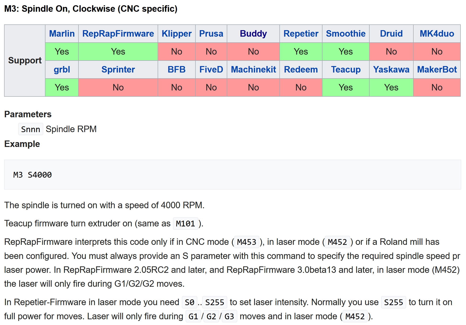
M3 GCode will do and what its expected parameters are, from the RepRap GCode Table — a community resource that is maintained by hand by volunteers.
Each of those codes is implemented in firmware, below I show the snippet of C++ that defines the switch for any “M” code — here I am looking at the Marlin firmware (a derivative of GRBL [20]) that is popular among hobbyist FFF printers. This snippet shows the compile flag HAS_CUTTER to define motion so even if we can find this snippet of code, we still won’t know if the firmware that is currently running on our controller has it set — we would need to look at the configuration file as well. This is not an issue when the value is properly represented in the reference table (Figure 2.3), but if we or someone else has modified the controller we would need to see the source code that was compiled and loaded onto the controller.
// in Marlin/src/GCode/GCode.cpp
// line 477
  case 'M': switch (parser.codenum) {
      // ...
      #if HAS_CUTTER
        // M3: Turn ON Laser | Spindle (clockwise), set Power | Speed
        case 3: M3_M4(false); break;
        // M4: Turn ON Laser | Spindle (counter-clockwise), set Power | Speed
        case 4: M3_M4(true ); break;
        // M5: Turn OFF Laser | Spindle
        case 5: M5(); break;
      #endif
      // ...
  }
// exit line 1172
So, the M3 from earlier went to case 3 to call M3_M4(false). The actual implementation of that function can be found deeper in the firmware source, with another selection of compiler flags (ENABLED(LASER_FEATURE)). The complete definition of that function is in Listing 2.3.
Firmware for GCode interpreters can be particularly difficult to understand because they contain functions like planner.synchronize() and planner.buffer_sync_block() which both relate to the machine’s acceleration controller; it is using a different time encoding for motion than what a pure interpolation across GCodes would generate. As I mentioned in Section 1.3.3, GCodes themselves are not encoded in time, but machines of course are. This means that interpreters are always managing multiple representations for actions they should take: one which is skewed according to the velocity optimization, and another which is not (yet). Understanding when something will actually be scheduled vs. when it is queued into the interpreter is difficult, because their internal representations in time are varying depending on what stage of the planning step they are in. For a more complete overview of velocity planning, see Section 4.2.4. In Section 2.2.4.8, I show some researchers who used an estimation of what this velocity planning step would do to their input GCodes to then encode their custom controls on top of that time encoding, to align the two representations. In MAXL, we also use time-based encodings to improve how modular code can interact with trajectories.
#if ENABLED() etc.
// in Marlin/src/GCode/control/M3-M5.cpp
void GCodeSuite::M3_M4(const bool is_M4) {
  #if LASER_SAFETY_TIMEOUT_MS > 0
    // Reset timeout to allow subsequent G-code to power the laser (imm.)
    reset_stepper_timeout();
  #endif

  if (cutter.cutter_mode == CUTTER_MODE_STANDARD)
    // Wait for previous movement commands
    // (G0/G1/G2/G3) to complete before changing power
    planner.synchronize();

  #if ENABLED(LASER_FEATURE)
    if (parser.seen_test('I')) {
      cutter.cutter_mode = is_M4 ? CUTTER_MODE_DYNAMIC : CUTTER_MODE_CONTINUOUS;
      cutter.inline_power(0);
      cutter.set_enabled(true);
    }
  #endif

  auto get_s_power = [] {
    if (parser.seenval('S')) {
      const float v = parser.value_float();
      cutter.menuPower = cutter.unitPower = TERN(
          LASER_POWER_TRAP, constrain( v, 0, CUTTER_POWER_MAX),
          cutter.power_to_range(v)
      );
    }
    else if (parser.seenval('O')) { // pwr in PWM units
      const float v = parser.value_float();
      cutter.menuPower = cutter.unitPower = CUTTER_PWM_TO_SPWR(
          constrain(v, 0, 255)
      );
    }
    else if (cutter.cutter_mode == CUTTER_MODE_STANDARD)
      cutter.menuPower = cutter.unitPower =
          cutter.cpwr_to_upwr(SPEED_POWER_STARTUP);

    // PWM not implied, power converted to OCR
    // from unit definition and on/off if not PWM.
    cutter.power = TERN(SPINDLE_LASER_USE_PWM,
                        cutter.upower_to_ocr(cutter.unitPower),
                        cutter.unitPower > 0 ? 255 : 0);
}; if (cutter.cutter_mode == CUTTER_MODE_CONTINUOUS ||
cutter.cutter_mode == CUTTER_MODE_DYNAMIC)
{ // Laser power in inline mode
#if ENABLED(LASER_FEATURE)
// M3 or M4 is powered either way
planner.laser_inline.status.isPowered = true;
get_s_power(); // Update cutter.power if seen
#if ENABLED(LASER_POWER_SYNC)
// With power sync we only set power so it does not effect
// queued inline power sets
// Send the flag, queueing inline power
planner.buffer_sync_block(BLOCK_BIT_LASER_PWR);
#else
planner.synchronize();
cutter.inline_power(cutter.power);
#endif
#endif
}
else {
cutter.set_enabled(true);
get_s_power();
cutter.apply_power(
#if ENABLED(SPINDLE_SERVO)
cutter.unitPower
#elif ENABLED(SPINDLE_LASER_USE_PWM)
cutter.upower_to_ocr(cutter.unitPower)
#else
cutter.unitPower > 0 ? 255 : 0
#endif
);
TERN_(SPINDLE_CHANGE_DIR, cutter.set_reverse(is_M4));
}
}This leads to another point, that GCode interpreters are buffered. In order to optimize over velocities, they need to look ahead. Whichever other system is sending them GCodes (sometimes a serial port, sometimes they are read from e.g. an SD card) is not always guaranteed to have exceptional bandwidth, and so interpreters must keep a number of moves in their queues, a bit larger than they may need to plan over. This makes it difficult to build interpreters that are responsive to new inputs: we can only insert new GCodes at the end of this queue, and must wait for previous inputs to be “flushed” (actually run) before the new command does anything. Many interpreters have simpler handles to (for example) change the velocity of the machine without waiting for a GCode to move through the queue, but we cannot change the spatial trajectory itself without halting and restarting the machine.
Based on this look at how a standard GCode is implemented, we can see what steps would be required to write a new GCode that extends machine operation:
- First, write the low-level firmware driver that runs the new piece of hardware. This may involve modifying an existing GCode interpreting control board (re-purposing some of its outputs and inputs), in which case the source code needs to be available. If the appropriate low-level drivers are not available on any of these boards, we need to develop a new circuit and firmware.
- Define a new GCode, picking something like
Mxxand ensure that the instruction does not collide with others in publicly available tables.- Write down what that GCode means,
- Integrate the new firmware with the existing firmware’s interpreter and planner. In some cases the additional compute power required by this new functionality may introduce issues at runtime.
- Integrate that new GCode with whichever program is being used to write machine instructions, either a CAM post processor or perhaps a custom Python code.
There are many better approaches to this problem in research communities that I will cover in the next sections (after a broader look at systems architectures more generally), but GCode interpreters remain extremely common in practice.
2.2.2 Background on Networks
2.2.2.1 Network Constraints and Benefits in Control
In Section 1.4.2 I mentioned that communication between control layers is a key constraint on our ability to partition systems in the ways we might like; controllers have bandwidth and timing requirements, but networks have bandwidth limits and delay. Operation over networks also requires some extra computing power to serialize, transmit, receive, route, and deserialize messages. This means that no matter how much engineering we do in our network layers, distributed controllers will always be less performant and less deterministic than monolithic controllers where all elements are in the same CPU.
For a simple example imagine a control loop that drives a motor according to readings from an encoder. We could build this using a distributed system with i.e. two \(48MHz\) microcontrollers (one CPU for the encoder and one for the motor) or in a monolithic system with one \(94MHz\) microcontroller performing both tasks. The second option will have superior performance because moving data from one process to another in the same CPU is always faster and more reliable than sending it over a network; network delay is directly related to controller bandwidth. Networks are also variable: if a link is congested its performance will decrease non-linearly (i.e. slowly at first and then all at once) 15. Out of band disturbances i.e. noise in the surrounding electromagnetic environment can cause packet loss16 and networks can be degraded by unrelated computing loads: if a microcontroller is busy computing new control values it has less time to process messages. So, network variability is directly related to controller determinism: moving data between two processes in one CPU is much more reliable than moving data across a network link. Each of these constraints is discussed in [21] and [22], and network performance is evaluated with regard to controller performance in [23]. These show that networks must be designed alongside controllers to understand total system performance.
On the other hand, the distributed controller in this simple example is more modular: we could re-use the encoder module with different motor drivers, or vice versa. This is sometimes a more valuable property than raw performance. In larger systems distributed controllers can provide pure performance benefits as well. For example if a controller needs to sample e.g. six different sensors before generating a new output signal it may be faster to distribute each of those sensor readings to a standalone microcontroller for each and then collect readings over a network. This is especially true where the total compute required by a control program exceeds the power that is available on any single microcontroller.17
The exact “break-even” point for these partitioning outcomes is dependent on constraints from the networks, the available CPUs, and the particular control task. The problem of optimal partitioning for distributed systems is handled directly by [24] for the general case (distributed computing tasks) and for realtime controllers in particular by [25].
Solutions to these problems also extend into our controllers’ mathematic architecture as well; we can “trade computation for bandwidth” by distributing predictive models throughout a system [26], relying on those models for intermediate estimates of distributed system states. Similar patterns appear when partitioning parallel algorithms over compute cores (using optimal partitioning to minimize memory contention [27]) and in edge computing for mobile device networks [28].
These ideas are most relevant in this work where we want to align motion control trajectories generated in one device with their execution in other devices. If they were fast enough, we could rely on network speed alone to synchronize devices. However, the links between path planners and motor controllers and sensors introduce real delay and indeterminacy and so we need to develop a strategy that will work well despite those limits. Each of the strategies that I cover in Section 2.2.4 manages this differently.
These constraints do not only apply to classically “networked” controllers: even monolithic GCode interpreters that receive new GCodes over i.e. a USB cable face the same issues. I expand on that in Section 2.5.2 alongside notes on how this background informs MAXL’s design.
Developing networks for real-time systems is a common challenge and so there is well established practice. For example OSAP borrows the “earliest deadline” scheduling pattern from [29] (see 2.3.1), and I use some key insights on clock synchronization from Network Time Protocol (NTP [30]), its high-performance counterpart Precision Time Protocol (PTP [10]) and other simple approaches for clock sync [31] [32]: using simple diffusion and control laws for clock discipline18 (see 2.3.2.2).
2.2.2.2 IP vs. FieldBus vs. Source Routing Networks
Much of our networks’ complexity comes from the routing layer. IP networks use “destination routing” where packets contain a destination address that is globally resolvable and the network itself resolves the route at runtime. To do this they keep tables that map ports to addresses and learn which ports point towards which destinations over time as they receive packets from those destinations. To forward messages routers read recipient addresses in packet headers, lookup which port those recipients are available on, and then copy the message onto the appropriate port [33]. Performing these steps efficiently can be complex and routing tables can consume large amounts of memory [34], [35] but in well-developed network stacks (i.e. the internet) the problem has been exceptionally well managed and is done one dedicated hardware [36], [37], [38].
Some efforts have been made to compress these algorithms for smaller devices [39] but many embedded networks instead use simpler busses where the routing step is skipped entirely, in networked control these are called FieldBusses, for example I mentioned CAN bus [5] as a primary example in the introduction to this chapter (2.1.2). On a bus, all devices receive every message and they simply ignore packets that are not intended for them. Some busses specify that each device on the bus has a unique address, whereas others ignore individual addressing entirely and delineate packets purely based on the data that they contain — i.e. the network model and data model are completely collapsed. Busses have a scalability downside because all devices need to share the same amount of bus bandwidth (they share one transmission “medium”) and a computing downside because each device needs to listen to, delineate and read each message even if those messages are not intended for them whereas point-to-point networks can be organized into subtrees of local traffic. Busses can also be less deterministic for this reason: if a number of devices try to transmit a packet at the same time their packets would collide, so each bus must develop a Media Access Control (MAC) strategy for collision avoidance. EtherCAT’s innovation was to use a bus network topology with a point-to-point “ring” link topology: packets travel along the ring where they are read by each device, and each device forwards them while inserting new data into the same packet [8]. They use standard Ethernet PHYs (Physical Layers) for this, but specialized Network Interface Controllers (NICs) to manage the low-latency packet forwarding / data insertion step. See Figure 3.11 and the surrounding text in Section 2.6.1.2 for more on that step. Busses have the advantage that devices can receive broadcast (aka multicast) messages in sync which is especially useful in control where we may want to synchronously send i.e. all motors in a controller new control values.
I should also note that switched Ethernet networks have also been adopted for networked control [40]. Switched Ethernet is an interesting example of the bumpy application of the OSI model and “sticky” / high inertia adoption of working technologies; Ethernet was originally developed in the 1970s for shared-media links over coaxial cables, and so it specifies that any device have a globally (as in, worldwide) unique MAC address. In large systems this led to the same scaling issues for shared-media busses that I mentioned above, and so switched Ethernet was developed where transparent switching devices are added between individually point-to-point Ethernet links. Like IP routers, these also learn and store routing tables in order to forward messages along individual links. This means that like EtherCAT, these systems look like a bus (and include multicast capability) but their physical topology is point-to-point, eliminating most of those scaling issues. Because switched Ethernet hardware was developed for wide use across datacenters and consumer networking, they are cheaper to integrate than EtherCAT and only slightly less performant. For a final note, Ethernet hardware is still challenging for a small microcontroller to operate and only high end \(\mu c\)’s have this capability, and even then require external physical layer hardware to actually drive the signal. Integration on switched Ethernet networks also requires that each device has a MAC address, and again not every microcontroller is given one - they are allocated to device manufacturers in address space blocks that must be licensed by the IEEE Registration Authority to maintain their global uniqueness.
One alternative to both is source routing [41]. This was first introduced to me by my advisor Neil Gershenfeld who developed a scheme called APA (Asynchronous Packet Automata), a description of which is in Nadya Peek’s thesis ([13] Section 3.1). In source routed networks, intermediate devices are mostly stateless; packets themselves contain routing instructions rather than destination addresses. This makes for simpler routers and networks overall and enables more precise network configuration, but requires that devices know where their recipients are because they write the routing instructions. This requires careful configuration and a deep understanding of the network, whereas destination-routed networking is simpler from the device programming standpoint; if you know your intended recipient’s address you just write that into the packet header and the job is done.
Source routing is used today where networks designers want explicit control over routing paths, simple and more robust router designs, and high performance. For example SpaceWire [42] source routes data between sensors, processing units and telemetry for on-orbit scientific instruments and is maintained as a standard by the European Space Agency. Source routing is especially important in space because it allows for the definition multiple routes between the same two endpoints such that if a device along one route flips a bit due to stray radiation the change can be detected and either corrected or retransmitted. The simplicity also makes it easier to deploy on robust and deterministic computing systems like FPGAs. SpaceWire is overall the most similar architecturally to OSAP among currently practiced network strategies, I make a more complete comparison between the two in Section 2.6.1.3. Source routing is also used in supercomputers to connect partitioned CPU cores [43] and in “network on a chip” systems for high performance interconnect of local processes [44], [45].
OSAP uses source routing for most of the same reasons: machine networks are local and so security is less of a concern, routers should be simple, performance is important, and direct configuration of routes is a valuable tool for the design of networked controllers as I’ve just explained in 2.2.2.1. In trading away complexity in the network, it does add some complexity to network configuration because routes must be configured using a view of the network topology that includes the transmitter and receiver (so that a router can be mapped between them). In OSAP, that goes hand-in-hand with the automatic detection of network topologies that is also useful to ascertain hardware configurations. I discuss that step in Section 2.3.2.1 and show how it is used in PIPES to connect software modules together in 2.4.4.3, where data routes for the program are written directly on top of source routes — this lets us directly configure network traffic at a program level.
Source routing is also related to strategies for larger scale network optimizations that I will discuss under the next heading (2.2.2.3), but it has fundamental security issues in open networks because transmitters have authority over where their packet lands; this vulnerability is what makes it uncommon for everyday networking.
2.2.2.3 Network Design as Optimal Partitioning
We can think of network design itself as an optimal partitioning problem, in Chiang’s excellent paper [46] network operation is explicitly framed as a distributed control problem that can be subjected to optimization-based design and operation. In this case, the problem is to choose where (i.e. in which protocol layer or in which device) different parts of the networking algorithms should go: for transport control, flow control, routing, etc. This is the framing that is adopted by the Next Generation Protocol working group [4].
In another view we also have the problem of optimizing traffic within a network, i.e. routing data flows over a constrained set of available paths. Source routing is one of the choice tools in this domain, it has seen a resurgence in carrier-scale network optimization where packets are partially source routed in a scheme called “segment routing” [47]. Network optimizations are also common in datacenters or in large local networks (on i.e. a university campus). This is where Software Defined Networking (SDN) is most common. In SDN, network topologies (maps!) are used by centralized planners to optimize flows within networks. This was originally introduced with OpenFlow [48], a tool that allowed network administrators to remotely configure network hardware by hand for efficiency experiments, but that capability quickly led to the development of “policy based routing” [49] [50] where optimal network flows are described declaratively by administrators and then configured with software that uses realtime data on network traffic to measure flows - a fairly explicit form of constraint-based optimization. These approaches are used extensively by i.e. Google [51] and Microsoft, whose overall datacenter architecture is described very well in [52] using policies from [53] and remotely reconfigurable FPGA routing hardware from [54].
OSAP and PIPES do not come anywhere near this level of complexity, but I think it is interesting to keep in mind as we design networks: again, we see a relationship between global system oversight for configuration and remote reconfiguration of lower level hardware for realtime operation - and of course the idea that constraint-based optimization of even the networking components in our systems is interesting.
2.2.3 Background on Distributed Programming Models
Next I want to look briefly at distributed programming models in a broader window, before focussing down in the next section on machine-specific architectures and programming models in 2.2.4.
There is a huge amount of work in this domain. I will try to show that most approaches here are suited either for high-level systems or for embedded systems; i.e. at the same realtime boundary where GCode sits. In these distributed systems, bridging across that gap is largely still done using middlewares.
The umbrella keyword for systems integration for hardware is Cyber Physical Systems (CPS), an up-to-date review of which is in [55]; this gives a sense of the breadth of concerns that are relevant for systems design. A major tension in the field is around determinacy, [56] notes that most of these systems are combined in a way that determinacy is not preserved, but shows that more complete descriptions of CPS could enable rigorous evaluation of their determinism. That means modelling networks, data flows, and computations within a system’s components - a fairly heterogeneous set of descriptors. A key challenge in this regard is ascertaining overall state in any given CPS. On the networking side this is related to the prior two sections where we looked at the importance of modelling networks themselves. At the application layer the focus is on “plug-and-produce” systems that propose automatic discovery of device descriptors and data models [57], [58].
2.2.3.1 Message Passing Middlewares
So, the key capability of these systems is message passing. This seems like it should be simple but it requires that messages are routed according to a system designer’s wish (which requires discovering network configurations and naming devices and messages) and that messages are encoded in a manner that each device can read and write them. There are four systems that are worth talking about in this regard, each with some subtle and some more substantial differences. These are each known as middlewares (see [59], Section 1.119 and the original description in [60]).
MQTT [61] is the simplest. Devices publish and/or subscribe (pub/sub) to “topics” that have human-readable names and payloads are routed using centralized “brokers,” it is most common in IoT networks and most payloads are serialized in JSON, but any binary format is possible. Network configuration is simple: each device is configured to point to the broker which normally has a static IP address.
ZeroMQ [62] has pub/sub semantics but is more akin to “sockets on steroids” (their wording), and is decentralized by default; devices can discover one another using multicast packets. ZeroMQ does not specify data formats, that is left up to the programmer.
OMG-DDS (Object Management Group’s Distributed Data System [63]) is most similar to ZeroMQ but does enforce data formats, which enables automatic discovery. In this system, programmers specify which data they will pub/sub to under a schema for typed topics (in the OMG-IDL, for Interface Definition Language) and then devices discover one another at runtime and send messages according to the schemas found in the local network (i.e. sending data to neighbors who specify that they would like to subscribe to their stream).
The OPC Unified Architecture (OPC-UA [64]) was developed specifically for industrial equipment and is most similar programmatically to OMG-DDS but includes built-in data schemas that are maintained by OPC. OPC-UA systems engineers can still define their own types, but the point of the specification is to enable interoperability using shared and standardized descriptors.
A key note is that each of these systems relies on IP-based network backbones and their devices’ local operating systems to operate those networks. To interact with hardware directly via embedded processors, bridges are developed that pass data over simpler link layers into operating systems that run these more advanced middlewares. See [65], [66], [67] and [68], and a direct comparison to OSAP’s inclusion of embedded devices in Section 2.6.1.2.
For a better look at these systems, this evaluation paper [69] summarizes their differences in more detail and measures relative performance (MQTT is the slowest overall, likely due to its reliance on the centralized broker). I should also note that DDS also has an extensive interface to configure Quality of Service (QoS) for each topic, i.e. specifying transmission deadlines, priorities and delivery guarantees - these are essentially transport layer configurations.
2.2.3.2 ROS: Application Layer Middleware via Message Passing
Of course we also have to talk about ROS, the Robot Operating System [70] - specifically the new implementation ROS2 [71]. It is a “a set of software libraries and tools” for robot applications; another middleware but its purpose extends beyond messaging alone to help robot systems authors integrate sensing, simulation, and planning softwares. In ROS, DDS is used for message passing but individual ROS “nodes” (blocks of software) expose pre-defined APIs using community standard20 message formats. Software packages in the ecosystem connect to one another through this framework and systems authors build custom applications by composing these packages, authoring their own middlewares to connect them. Representations of physical robots are built using REPs (for ROS Enhancement Proposals), which are more formal standards to describe robot kinematics and i.e. units of measurement. To connect to hardware, ROS also provides a litany of drivers, these are ROS nodes that wrap existing OS-level interfaces to devices and exposes them as ROS topics, services and parameters.
In many ways, ROS is similar to GCode: it is a middle layer between hardware and software that is built using convention but is not strictly typed or inspectable. Using ROS is a practice and requires users have some tacit knowledge of its internal architecture, principles and conventions [72]. One-third of ROS bugs are dependency errors [73] that arise from hidden misconfigurations where node or user-code is set up according to varying or out-of-date conventions [74], discovery of configurations is not itself built into ROS, but some work adds additional tooling for this [75] [76].
2.2.3.3 Serialization Layers
Each of these middlewares must serialize messages: this means taking data out of memory in the transmitter’s CPU and writing it into a format “on the wire” that can be read by the reader in a standard format.
The most common serialization format is JSON (JavaScript Object Notation), which serializes structured data into human-readable strings. It is commonly used in MQTT and is extremely flexible, but serializing strings is computationally expensive and also memory intensive [77]. More performant systems use compiled data protocols like ProtoBuf [78] or Capn’ Proto, both of which are compared in [79], [80]. These are exceptionally performant but rely on shared schemas that are built before systems are compiled: programmers must specify data types ahead of their use and without access to these schema (i.e. in a .proto file) it is difficult to inspect them remotely, although they do provide tools for automatic documentation and some extensions allow for runtime reflection on types.
2.2.3.4 Dataflow for Hardware
There are three systems worth discussing that each implement dataflow programming models for hardware.
LabVIEW is the longest standing and most widely used dataflow tool for hardware. It was developed by National Instruments for the development of new laboratory equipment and allows scientists and engineers to compose programs using a mixture of software components with “virtual instruments” [81]. Virtual instruments are implemented in much the same way as other embedded devices described in the subsection above on middlewares: OS-level drivers communicate with hardware via bridges over USB, serialport or custom communication layers and expose those devices within the LabVIEW runtime itself via an “agent” that virtualizes them. For this reason it, like others, is limited in computational scalability by the one standalone dataflow runtime: messages queued between two hardware instruments must pass through this domain through those bridges.
Node-RED is used in IoT [82] [83] to compose software for “collecting, transforming and visualizing data.” It ingests messages over MQTT or HTTP and can broadcast transformed data over the same protocols. Systems are composed in flows where each block is a wrapper on a JavaScript function or class. While it connects to distributed devices, it is not itself distributed: blocks operate in a single runtime. Connecting two node-red runtimes into one system requires that each manually configures MQTT inputs and outputs, and that those be configured to communicate with one another, and discovery of the global system from some other location is not possible.
MsgFlo [84] also runs on MQTT (or AMQP: Advanced Message Queuing Protocol [85]) but is more distributed: each process / device is independent and can receive or transmit message flows, capabilities of remote devices can be automatically discovered, and dataflow graphs can be composed across those devices. MsgFlo is most similar to PIPES in this regard, but differs in a few key ways that I will explain in Section 2.6.1.5.
2.2.3.5 Patterns from the Web
Each of these more modern approaches to distributed systems borrow heavily from design patterns that were originally developed for the Web, the largest and messiest distributed system of all time! There are three relevant ideas that I would like to cover.
The first is organized around REST for Representational State Transfer, introduce by Fielding [86], [87]. This is a widely-used architectural style for web APIs that encourages simpler interoperation of online services. It encourages a few key principles: statelessness in the interface, layering of server functions, and unified interfaces using Unique Resource IDs (URIs) and a core set of operations. The style itself doesn’t specify anything about the particular implementation, but it is most often followed for HTTP messaging on the web where the core operations are: GET (read), POST/PUT (create or update), PATCH (partial update) and DELETE. Each request is made to a resource endpoint (a URI) alongside the operation keyword, a header (metadata and context, i.e. state) and a body (the payload). In many ways, REST APIs are the middleware of the web.
A common programming framework for RESTful APIs is the Model-View Controller (MVC) originally developed for the smalltalk language [88] they are widely adopted in web applications [89]. Here the model is whichever underlying representation is being interacted with: a database or user session on the web or (in the case of PIPES) a machine configuration. The controller mediates between the user and the model i.e. allowing and implementing or denying requests to make changes to that model, and the view is what is rendered for the user.21 OSAP and PIPES both use this framework; controllers in each system return views of their local models for network state (via OSAP, 2.3.2.1) and for program state (via PIPES, 2.4.4.1). These are then combined into a global view of the PIPES system model (Section 2.4.4.1), which is the main interface for programming in PIPES systems.
RESTful APIs are often used by microservice style server architectures, where requests made to datacenter-scale systems are handled using modular systems composed of smaller programs, each of which provides some subset of the contents of the reply [90]. These allow more rapid development of server programs because components can be replaced piecewise and i.e. authored in different languages: in fast cpp for complex tasks or in scripted languages like JavaScript or Python for simpler or rapidly developed features. The same is true for updating large distributed systems: rather than updating the entirety of a system’s code at once, individual instances in the stack can be updated one at a time or i.e. tested partially before deploying completely. Microservices also allow for systems-scale optimization of compute resources: rather than loading one monolithic piece of code in each server, services can be spun-up depending on which are needed most often according to current loads. This level of configuration connects to network-scale optimizations discussed in Section 2.2.2.3 where data flows are optimized between processes, at this layer the actual layout of those processes can be orchestrated. So, again, we see this correlation between the optimization of program and network configurations in distributed systems and their coupling.
For one final note in relation to the economic partitioning of systems and how that relates to technical partitionings (from Section 1.4), microservices also serve to bundle organizational capabilities into standalone software components; teams that are responsible for a particular component of a firm’s technical systems are also responsible for its integration into their server’s backend via a microservice (see [56], Section 3.1). This simplifies organizational complexity within the firm: that team does not have to explain their system’s internal organization to their collaborators - they just have to specify the interface. This idea is carried into OSAP / PIPES and MAXL: in Section 8.3 I relate the architectural choices made in these systems to the same organizational complexity tasks faced in open source hardware.
2.2.4 Background on Machine Control Architectures
Continuing on a path away from pure architectural background through real systems, in this section I want to discuss a few common machine control architectures from industrial control to hobby 3D printing and in related research. Under these headings I will discuss how each is arranged computationally (i.e. which controller function is located in which computing device) and how those arrangements relate to the myriad ways that programmers and users configure and operate machine systems.
2.2.4.1 Centralized, Monolithic Control
The simplest and most common arrangement is the monolithic / centralized GCode interpreter. One of these is shown in Figure 3.1 on a Prusa FFF Printer [91]. These boards run a single firmware that consumes GCodes via a serialport, WiFi or an SD Card. They interpret those codes, queue them into buffers for velocity planning (see Section 4.2.4 for a longer explanation of the velocity planning step), and continuously update their queues and velocity plans as they simultaneously operate hardware like stepper motor drivers, heaters, and spindle controllers via low-level drivers.
2.2.4.2 Centralized Timing and Control with Remote Devices
In most state-of-the-art industrial machines a central microcontroller or PC running a realtime operating system performs computational tasks like GCode interpretation, velocity planning, and some components of servo feedback control and sends commands to motor driver hardware over simple network links or fieldbusses like EtherCAT.
Drive commands can be sent in a variety of forms. Splines are sometimes used because they cleanly encode position, velocity, and acceleration signals and can be interpolated at rates that exceed the network’s bandwidth. I rely on splines in MAXL for the same reason (see Section 2.5.3). Some systems transmit piecewise linear segments for motor interpolation, and others send simpler sample-and-hold reference signals for motor velocity. In each of these cases, a faster controller in the servo drivers themselves operates the motor hardware at much faster bandwidths, normally between 500 and 2000Hz depending on the system dynamics.
These networked controllers are very simple distributed systems but rarely deploy the types of middleware that I surveyed in Section 2.2.3, instead they write simpler communications layers between GCode interpreters and fieldbus protocols.
This pattern is being adopted in open source, especially by the Duet ecosystem [17] which runs RepRapFirmware [18] and uses a CAN fieldbus to connect interpreters to auxiliary drivers; the Duet mainboard is still mostly a monolithic controller but can be extended under this pattern.
2.2.4.3 Object Oriented Hardware
I briefly introduced OOH from Peek [13] and Moyer [12] in the very beginning of this section (2.2). These controllers virtualize control and configuration by moving core logic into an OS where machines can be programmed using virtual representations of hardware and machine control. It also eschews GCode interpretation and instead presents a more modular machine API that can be used to develop machines as realtime-interactive devices and to better integrate motion control with user applications.
OOH’s main innovation is in the way machine configurations are expressed as modular software APIs, overlaying object oriented programming with modular hardware objects. Peek shows in [13] how this framework can be used by new machine designers to configure and control hardware of their own design using more flexible representations of machine control and interacting with controllers dynamically via Python scripts.
In terms of computational partitioning is would also fall in the class above: it centralizes program interpretation and velocity planning and sends lower-level motion segments to motors over a fieldbus. In this case the fieldbus is a custom implementation called FabNET.
2.2.4.4 Klipper
Klipper [92] is an interesting hybrid system that follows most closely in-line with Object Oriented Hardware controllers.
Klipper’s main logic (GCode interpreting, velocity planning and optimization of stepper motor pulse timing) runs in the Linux operating system and is normally deployed on small single-board computers (SBCs). It’s use of higher power computing available in SBCs enables it to build more advanced controllers; Klipper was the first open source system to implement input shaping, a filter-based velocity planning step that minimizes excitations of machines’ resonant modes (see Section 4.2.5 for background on input shaping).
Klipper is fundamentally based on step-and-direction based control of stepper motors. Precise and high bandwidth timing of these step pulses is required to smoothly operate stepper motors, the likes of which are difficult to generate within an operating system. Klipper offloads this control component (and control of other auxiliary hardware) to embedded devices and communicates with them over USB links using a custom and very low level protocol. This allows Klipper systems to operate stepper motors’ step and direction pins at extremely high frequency,22 \(223 \text{kHz}\) on SAMD21 microcontrollers (with a \(48 \text{MHz}\) clock) and up to \(885 \text{kHz}\) on RP2350 microcontrollers (a more modern device with a \(150 \text{MHz}\) clock) [93].
While it is authored in Python and so easier to edit, Klipper is still a GCode interpreter and so extending it to modify control logic itself is nontrivial. Configuration is similar programmatically to other interpreters (a static config.py file containing controller parameters and options is modified) but is simpler to update because it does not require that the interpreter be re-compiled and re-flashed into firmware.
2.2.4.5 Urumbu
Urumbu was developed by my collaborator Quentin Bolsée and my advisor Neil Gershenfeld [94]. Like Klipper and OOH, it centralizes program state, configuration and velocity control into a Python program running on an operating system. Urumbu uses Python threads to increase performance of this software and in doing so can perform even very low-level timing of stepper pulses there without a realtime OS; one of the threads runs a tight loop that uses the OS clock to coordinate steps. It connects to devices over USB links using USB hubs and sends single-byte instructions to motors and sensors.
This makes embedded device development incredibly simple: each only has to translate single bytes into hardware outputs. For stepper motors, this amounts to one step per instruction using a bitmask where the 7th and 8th bits in the byte correspond to the stepper driver’s step and direction pins. Devices can optionally send one return byte in each cycle to read i.e. switch states. However, it limits performance according to the operating system’s USB driver performance. While this can be surprisingly fast (at \(2000 \text{Hz}\)) it is not deterministic and the low-level representation means that stepper motors’ stepping rate is limited to this frequency whereas high performance stepper drivers operate well above \(100 \text{kHz}.\)
2.2.4.6 StepDance
Ilan Moyer’s StepDance [95] is a motion control framework that aims to help machine designers develop new automated and real-time interactive machine tools, with a particular focus on craft-aligned interactions.
StepDance is similar to MAXL in that it describes machine controllers as flows of data streams that can be declaratively mapped and that controller configuration is based mostly on the arrangements of these flows. It also includes a library of dataflow blocks for kinematic transforms and function generators, a-la MAXL’s own set (in 2.5.4). Rather than encoding motion in basis splines, it uses pure step and direction streams. It runs entirely in firmware at a core step tick rate of \(25 \text{kHz}\) but multiple modules can be connected together using a custom physical link that encodes multiple axes of step and direction using pulse-width multiplexing over four-conductor audio cables. In earlier work by the same authors [96], a similar system based on step and direction signals is mixed with a classical GCode interpreter and velocity planner (Duet3D [17]).
StepDance is architecturally novel, it partitions motion control over multiple devices at extremely low latency by eschewing networks entirely. Instead they build a custom physical link that is packet-free; each digital pulse on this link encodes step and direction directly, although they do use pulse width multiplexing to encode multiple channels per physical link. The architectural through-line is to align the whole system around stepper motor drivers’ core representation for motion (discrete increments… steps) and broadcast those through a new network and software architecture.
That is perhaps also its weakness: these links cannot transmit arbitrary network data that would enable remote software control of kinematic blocks via i.e. remote procedure calls or interfacing with more traditional user interfaces or remote configuration tools. Control of inputs and outputs that are not step-based is also requires some extra steps, but they are well managed using i.e. a software block that converts analog inputs to steps using a velocity model and another that can convert step and direction integrated positions to a hobby servo’s reference signal.
In Section 7.4 I discuss the relative benefits and trade-offs that emerge when we use splines as a core representation, including the ability to use the spline’s natural derivatives for velocity and acceleration for improved closed-loop tracking, how spline representations allow for improved stepper interpolation, and their natural relationship to underlying machine physics.
Another difference between StepDance and the network-based controllers in this chapter is that we can re-create the control graph’s state remotely by inspection over the network to produce a global system model (2.4.4.1). Understanding global configuration of a StepDance system would require understanding each module’s source code and physical link mappings.
However, StepDance’s realtime performance surpasses that of the systems in this chapter, it’s \(25 \text{kHz}\) is equivalent to only \(40 \mu s\) delay. In Section 2.7.9 I show that in the stackup of MAXL, PIPES and OSAP the equivalent delay between two embedded devices is about \(400 \mu s\) or a \(2.5 \text{kHz}\) update rate, see Section 2.7.9 for a complete workup of timing results from this work. However, this is in the case where we are updating basis spline control points, so it represents an update rate but not an interpolation (stepping) rate, whose performance would be dependent on the interpolating module’s performance. In practice, I run the stepper motors (from 4.4) closed loop update at \(15 \text{kHz}\) which requires substantially more computing power than just stepping. But I also push most control elements into the operating system, and MAXL is based on a deterministic timing gap (see Section 2.5.2) between the OS and path execution. I discuss this also in 2.7.9: real-world delays due to this gap are typically \(64 ms,\) this is only \((15.625 \text{Hz})\) and above the threshold for human-perceptible delay for interactive computer systems i.e. drawing on a tablet with a stylus [97], but under the threshold for closed-loop teleoperation of robotic systems through the human visuomotor loop which is around \(250 ms\) [98].
2.2.4.7 Computational Control of Machines via GCode Wrappers
Many researchers choose simply to wrap GCode interpreters in improved, dynamic APIs. These are normally Python codes that connect to interpreters over a serial port, they expose a computational API on one side and write GCodes into the interpreter on the other. Frikk Fossdal in [99] and [100] develops interactive machine interfaces in Grasshopper (a dataflow programming tool that is integrated with CAD) using a Python script as an intermediary to send GCodes to an off-the-shelf machine controller, it also reads machine configuration states from the controller using a separate link available in the Duet3D ecosystem.
Hannah Twigg-Smith’s Dynamic Toolchains [101] and Peek and Gershenfeld’s mods [16] systems also use dataflow to control machines, but more indirectly: they are designed to write toolpath plans in a more modular fashion, but then render those toolpaths as GCode (mods and Dynamic Toolchains) or machine knitting instructions (Dynamic Toolchains) and transmit them to interpreters in off-the-shelf machines.
In Jasper Tran’s “Imprimer” system [102], computational notebooks are used as an interface for machine workflows: their system also implements an intermediary software object that communicates with off-the-shelf controllers using GCode, but presents a more useful API to the notebook and uses an additional intermediary representation to keep track of machine state.
The Jubilee project [103] [104] is a machine platform that implements a modular tool-changer, and has been successfully deployed by researchers to automate duckweed studies (a popular model organism) [105] and to study nanoparticles [106]. Jubilee also uses an intermediary Python object to interface with an off-the-shelf GCode controller.
Each of these works shows the value of integrating motion systems with application-layer scripting languages, but they are sometimes limited by the integration strategy. At the configuration level, each Python interface in these examples must mirror the GCode interpreters configuration in its own local state, this process is done by hand and misalignments can cause difficult to diagnose errors. Consolidating configuration state was a topic discussed during and NSF sponsored workshop that I attended on open source lab automation tools [107] where we used Jubilee machines to build new workflows. In terms of motion control, it is difficult for these tools to interact directly with as-planned machine trajectories because the GCode interpreters do not expose those. Besides the configuration challenges that can be resolved with careful engineering, this is not a real issue for the duckweed and nanoparticle studies or in any other case where moving to a position and then performing the new automation while the machine is stopped is sufficient, but presents challenges for researchers who integrate new process physics like those in the next subheading here and introduces delay and possible errors in shared digital representations of these machines. Each of these studies is also motivated by the idea that machines should be easier to modify for non-experts, so improving the configuration step remains important especially if we would like to apply them on a broader set of individual machines, each of which has a unique configuration.
2.2.4.8 T-Codes and FullControl
Two groups of researchers working on control of fluidic 3D printers [108], [109] have developed time-encoding (T-Codes) based machine control layers in direct response to the issues that I discussed in Section 1.3.3, which is that GCode interpreters’ velocity planners make it very difficult to synchronize additional axes of control with motion without modifying those planners directly.
These researchers want to control their custom gel extrusion printers using a system of their own design because off-the-shelf GCode interpreters for 3D printers make assumptions about flow dynamics that their systems do not contain. To work around this, they follow a few steps:
- Write a standard GCode for multi-material 3D printing.
- Strip that GCode of extrusion information, leaving only positioning commands.
- Use their machine’s acceleration and velocity parameters to calculate an exact time mapping between the original GCodes and the machine’s actual operation.
- Use that time mapping and the original GCode instruction to generate TCodes (time-encoded instructions) that operate their custom extrusion system.
This is an interesting approach and solves a classic type of problem that I have described already: of integrating new physics into existing motion systems. In Chapter 5, I show how the motion controller from Chapter 4 is more fundamentally modified to encode and then optimize both flow and motion physics together. Their insight is that machine operation is basically time-based, not position based and so external control should be orchestrated as such. This is present in MAXL’s use of fixed time encodings for basis splines, and in [110] I even showed a very similar example in synchronizing LEDs with velocity-controlled motion paths using time encodings of an “event” track type, the output from that experiment is in Figure 2.13.
Other researchers simply write computational APIs that can compose GCodes directly. One popular tool for this practice is called FullControl [111] and Blair Subbaraman extends the p5.js ecosystem in a similar tool [112]. This approach is excellent for more direct operation of hardware, but is mostly suited to experimentation, education and creative practice. However, it does show that while GCodes present certain integration issues, they still expose a relatively straightforward “API” that can be extended in simple and productive ways.
2.3 OSAP: Machine Systems Interconnect
Open Systems Assembly Protocol
OSAP (for Open Systems Assembly Protocol) is a relatively lightweight piece of software that I have authored in C++ for embedded devices and in Python for high-level system components. It includes a runtime where messages are queued and handled (Section 2.3.1) and software interfaces that connect that runtime up into software and down to network drivers (2.3.1.2).
Because it mediates between hardware and software and does so across networks (where the real “underlying hardware” is the network itself), it is akin to a distributed operating system. In contrast to most distributed systems architecture from the state-of-the-art, embedded devices are first-class citizens in this scheme.
Another main differentiator is that OSAP’s networking is link agnostic, meaning that it can be extended across many types of network technologies with relatively little overhead. Links are added to OSAP’s runtime in the same way that software is: via interface classes in Python (through composition) or in embedded (via class inheritance); to improve performance of networking hardware software interfaces are often missing between OSI layers, but OSAP includes them to improve systems-level composability. Links are all point-to-point at the moment but the protocol could be extended to include fieldbusses and includes reservations for this.
Because OSAP is a protocol and design spec, it should be easy to author in other languages when i.e. we want to build versions that provide handles to software written in Rust or JavaScript, or even into hardware design languages for custom silicon or FPGAs. At the moment I run it in Python and in embedded C++, but earlier versions were also written in JavaScript.
OSAP’s main task is to get serialized messages from any port in the system to any other port in a timely manner. It does so using source routing, a simple networking scheme that I discussed in Section 2.2.2.2 - OSAP’s implementation is described in Section 2.3.1.3.
It also provides two valuable services. Section 2.3.2.1 describes the discovery service which allows any device to retrieve a network map of locally connected devices. This allows us to inspect networks and determine i.e. if the motor drivers that our machine needs are, in fact, connected, how to reach them, and how to describe the network route between two other remote devices if we would like to remotely configure dataflows. Section 2.3.2.2 describes the time synchronization service, which keeps device clocks in step with one another. This is a critical building block for mechatronic systems since it lets us synchronize motion, measure real network performance, and collect coherent time series data from networks of sensors and actuators.
OSAP is the connectivity layer, programs are assembled within OSAP networks using PIPES (Section 2.4), and motion controllers are composed in PIPES using MAXL (Section 2.5).
In my description of OSAP in this section I first cover how it operates under the Runtime header 2.3.1; its structure in 2.3.1.1 and main components: ports and link gateways, and the software interfaces that are used to integrate them to the runtime (in 2.3.1.2), and then the networking scheme in 2.3.1.3: this describes how packets move through the network. Memory allocation, flow control and scheduling are all closely related and are covered in Sections 2.3.1.4, 2.3.1.5 and 2.3.1.6. We can then understand OSAP’s main loop in Section 2.3.1.7 and finally discuss the transport layer in 2.3.1.8. Network discovery (Section 2.3.2.1) and time synchronization (2.3.2.2) are both under the Services header, Section 2.3.2.
2.3.1 Runtime
At the core of OSAP is a runtime that manages parallel operation of network links and message passing and software modules that are attached to its ports. In embedded devices where no operating system is present, it resembles an RTOS (realtime operating system) because it allocates CPU time across software modules that each run sub-programs (this is scheduling). In workstation computing it runs within Python’s existing asyncio loop that itself runs within the existing OS. Below I describe its core data structure, its operating principle across scheduling, flow control and memory allocation, and the software interfaces that are used to connect it “down” into network segments and “up” into software.
2.3.1.1 Structure, Setup, and Loop
OSAP’s internal structure has three key elements:
- A list of ports, which are interfaces to software.
- A list of link gateways, which are interfaces to network segment drivers.
- A stack of packets to handle.
These are the software handles used by the runtime to schedule operation, receive and process packets, and collect information about itself during network discovery steps. Each is explained in more detail in subsequent sections. The runtime itself also has a few properties:
- A name, which can be remotely re-written, and is saved into non-volatile memory.
- A type name.
- A runtime version number and build type.
- A netresponder class on the 0th port (see 2.3.2.1).
OSAP is deployed as a software library that connects to device-specific drivers for i.e. link layers and other hardware through it’s own API. Those interfaces are defined in the next section on ports and links. I show how the runtime object itself is instantiated in embedded devices in Listing 2.5 (in the Arduino style) and in Python scripts in Listing 2.6. The notable difference is that the embedded runtime is currently limited in it’s ability to dynamically instantiate link gateways and ports, although I did implement that functionality on microcontrollers in an earlier predecessor to the system in my master’s thesis [113].
// in 'main.cpp'
OSAP_Runtime osap( // instantiate the runtime,
    "loadcell_cs5530_d21", // device type
    DEVICE_NAME // device name
);

// ... link instantiations
// ... port / pipes function instantiations

void setup() {
    osap.begin(); // initialize the runtime,
}

void loop() {
    osap.loop(); // call the runtime's loop repeatedly,
}asyncio. Link gateways can be instantiated dynamically or set up at the beginning of the program, which is what I do here: AutoUSBPorts() scans for and opens any USB-CDC devices that present with device IDs that are likely to contain OSAP runtimes. It does not matter which COM / tty number they associate with in the OS because systems configurations will be automatically laid on top of these network addresses later on. This utility also instantiates the MetaManager, which builds the PIPES Systems Object Model (Section 2.4.4.1) via network scan.
async def network_tools_setup(runtime_type_name, runtime_name):
    osap = OSAP(runtime_type_name, runtime_name) # runtime software object
    loop = asyncio.get_event_loop() # hook to the script's asyncio loop,
    loop.create_task(osap.runtime.run()) # attach osap's loop as a task

    auto_ports = AutoUSBPorts() # discover and start ports
    gateways = await auto_ports.start_ports()
    for gateway in gateways:
        osap.link(gateway) # attach

    manager = MetaManager(osap) # the PIPES SOM generator
    await manager.refresh_system() # perform the first scan

    return osap, manager
2.3.1.2 Ports and Links
I think of OSAP’s ports as facing up into software23 and link gateways as facing down or out into network segments and Figure 2.4 and other diagrams in this section reflect that. Both are attached to OSAP’s runtime using software defined interfaces. In C++ these are based class inheritance and in Python via composition. I show base classes in C++ for each in Listings 2.7 and 2.8 below; functions marked with virtual are implemented by the inheriting class and others are defined within OSAP.
Both interfaces have functional equivalents to network transmit and receive; for ports this means passing data across network routes to another port in some other runtime or, where the route is empty, to another port in the same runtime. For link gateways this simply means framing and sending data over its connected segment, or ingesting data from the same and adding it to OSAP’s internal message stack, which is described in the next subsection.
Almost any link technology can be added to OSAP, but each needs to perform a few key functions. The first is to encapsulate outgoing packets and delineate incoming packets from raw byte streams (this is “packet framing”), and the second is to ensure that packets written into OSAP’s message stack (see the next section) do not contain errors: OSAP’s internal operation is not robust to corrupted data. This is a common pattern across many network architectures.
These are not complicated tasks, for example in most of the systems that I used in this work, I promote simple UART drivers (which are ubiquitous and simple) into robust network links using Consistent Overhead Byte Stuffing (COBS) [114] to frame packets and also adding Cyclic Redundancy Checking (CRC) [115] for error detection. Specifically I use CRC16 CCITT with the 0x1021 polynomial as specified by [116] (a standard). COBS is designed for deterministic performance and CRCs can be calculated quickly using pre-computed tables. Doing both in firmware does introduce some computational burden, but the simplicity over using external network controllers or other ASICs for the task is advantageous, in Section 3.4 I expand on why that is the case.
class VPort {
  public:
    // Start / Run
    virtual void begin(void);
    virtual void loop(uint64_t now);

    // Software->OSAP (TX)
    boolean clearToSend(void);
    void send(
      uint8_t* data, size_t len,
      Route* destinationRoute,
      uint16_t destinationPort
    );

    // OSAP->Software (RX)
    boolean clearToReceive(void);
    virtual void onPacket(
      uint8_t* data, size_t len,
      Route* sourceRoute,
      uint16_t sourcePort
    ) = 0;

    // Constructor
    VPort(
      OSAP_Runtime* _runtime,
      const char* _typeName,
      const char* _name
    );

    // Properties
    char typeName[TYPENAMES_MAX_CHAR];
    char name[PROPERNAMES_MAX_CHAR];

    // States
    uint8_t currentPacketHold = 0;
    uint8_t maxPacketHold = 2;

    // Stash
    static uint8_t _payload[PCKT_MAX];

  private:
    OSAP_Runtime* runtime;
    uint16_t index;
};class LinkGateway {
public:
// Start / Run / State
virtual void begin(void);
virtual void loop(void);
virtual boolean isOpen(void);
// OSAP->Link (TX)
virtual boolean clearToSend(void);
virtual void send(
uint8_t* data,
size_t len
) = 0;
// Link->OSAP (RX)
void clearToReceive(void);
void ingestPacket(VPacket* pck);
// Constructor
LinkGateway(
OSAP_Runtime* _runtime,
const char* _typeName,
const char* _name
);
// Properties
char typeName[TYPENAMES_MAX_CHAR];
char name[PROPERNAMES_MAX_CHAR];
// ------------ States
uint8_t currentPacketHold = 0;
uint8_t maxPacketHold = 4;
private:
OSAP_Runtime* runtime;
uint16_t index;
};In many cases OSAP uses this link interface to virtualize existing network segments. For example we can establish OS-level software sockets and encapsulate those as link gateways in a runtime, the same is true of USB-CDC connections. In these cases and others, the underlying links already perform both or some of these tasks and so we do not need to re-define them in the link gateway’s driver. Sockets are already packetized and error corrected, whereas USB-CDC streams are unencapsulated but error corrected; in the underlying USB drivers they are also encapsulated, but these lower layer drivers are more difficult to write whereas USB-CDC drivers work “out of the box” on most operating systems. So you can see how the OSI model becomes somewhat strange here: we are taking IP-based sockets (a full network stack) and exposing them to OSAP at the link layer.
USE_UART_LINK to define which gateways the runtime will load.
// instantiate the USB-CDC gateway,
#ifdef USE_USB_CDC_LINK
OSAP_Gateway_USBCDC_COBS<decltype(PA_USB)> serLink(
    &PA_USB, // link driver
    "usb" // link type
);
#endif

// or instantiate the UART gateway,
#ifdef USE_UART_LINK
OSAP_Gateway_UART_COBS_CRC16<decltype(PA_SERIAL), true> uartPA(
    &PA_SERIAL, // link driver
    UART_BACKPACK_BAUD, // data rate
    "uart_rs485_pa", // link type
    PA_PIN_GP1, // link hardware configuration
    PA_PIN_GP0,
    PA_PIN_CS
);
#endif
This is a design choice based on the availability of these technologies to a systems integrator. OSAP is a kind of melting pot and these interfaces homogenize messy systems to make its internal system smoother; at the runtime layer each link gateway or port is like any other. This means that configurations for software-defined links — i.e. the COM number for wrapped USB-CDC connections or addresses for IP-based sockets — are external to OSAP. This is a design choice that increases simplicity of the networking scheme, but it limits our ability to configure networks remotely. There is future work planned to add these capabilities in a manner that doesn’t add complexity to the runtime itself (in Section 2.9.1.1), or to instantiate embedded link gateways based on the Knuckles Backpack ID Pin to update software configurations based on hardware state — see Section 3.3.
2.3.1.3 Networking and Packet Structure
OSAP is based on source routing. I covered a wider background on the strategy in Section 2.2.2.2; the basic scheme is that data sources write network routes directly into the packet header rather than specifying a destination address that must (1) be globally unique in the network and (2) be resolvable by intermediate network devices. Source routing is much simpler because intermediate devices simply read routing instructions from the packet (no thought required), but requires an outer loop of route configuration. In this work, that is done globally by way of OSAP’s discovery service (explained in Section 2.3.2.1) which is used at a programming level in PIPES to overlay software configurations on networks, see Section 2.4.4.3 on connection configuration and Section 2.4.4.1 for the Systems Object Model that represents those configurations (and underyling networks).
Figures 2.4 and 2.5 diagram two OSAP systems and examples of some source routes between ports. Operation of these routes is described below.
Packets headers contain small bytecodes that are interpreted by the runtime in order to forward messages, process them internally to provide network services like time synchronization, or send them on into ports.
Because link gateways and ports in a runtime are stored in ordered lists, each has an index — these are used in packet arguments. For example one of these instructions is link_forward, it has one argument for the link index that the message should be sent along.
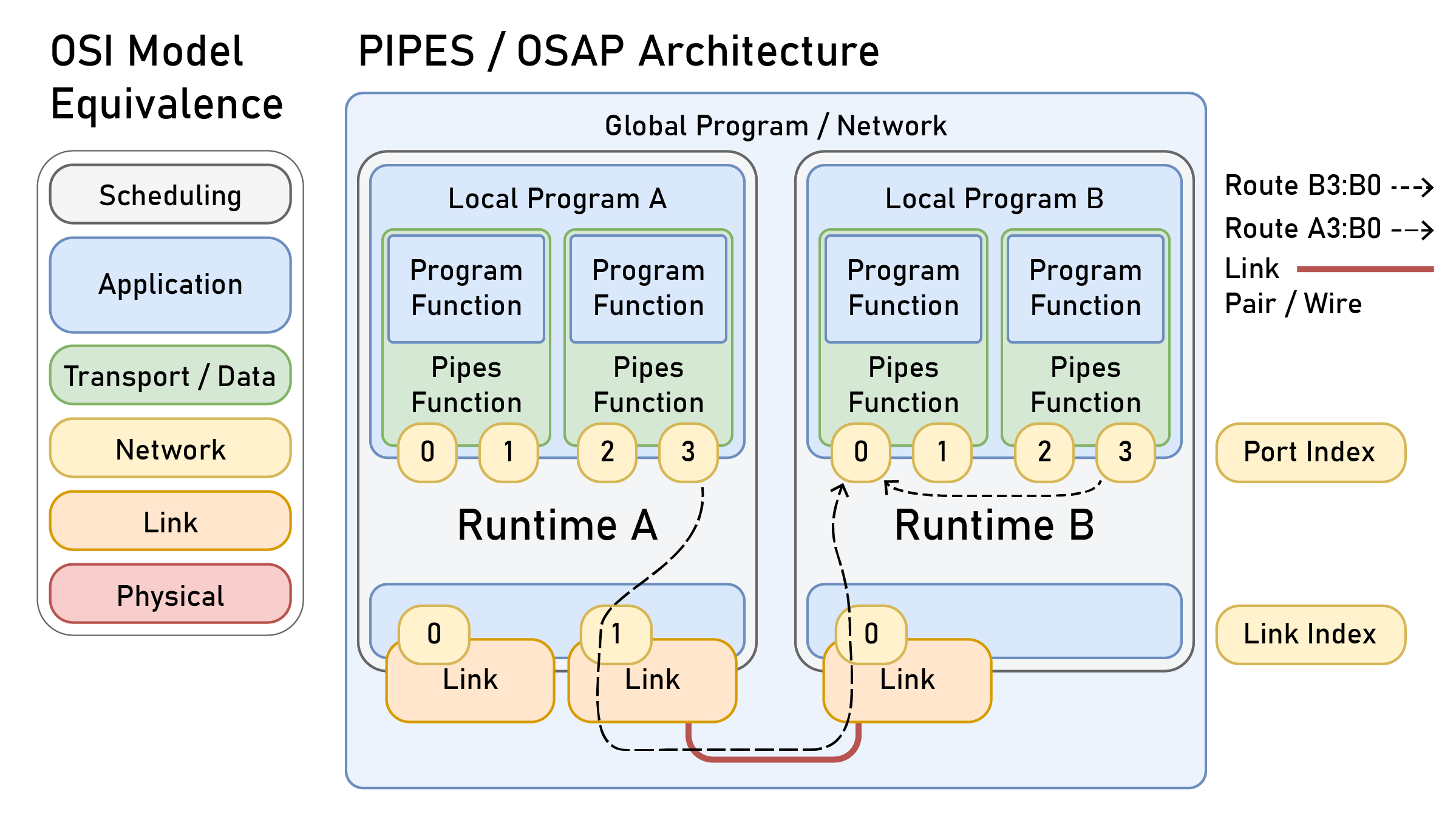
A and B each containing a local program and program functions that are wrapped as Pipes Functions. Link gateways and their indices are “below” the runtime, with functions attached via ports “above.” Each of these have indices, which are used in packet routing. Two routes are shown and routing instructions for each are shown in the text below.
| Route | 1st Bytecode | 2nd Bytecode |
|---|---|---|
| B3:B0 | port_handle(src: 3, dst: 0) |
|
| A3:B0 | link_forward(1) |
port_handle(src: 3, dst: 0) |
| B0:A3’ | link_forward(0) |
port_handle(src: 0, dst: 3) |
The first byte in the packet is the instruction pointer, it indicates the in-packet location of the next instruction. The instruction type is indicated by the first two bits of this byte, so to get the opcode we simply do:
// the instruction pointer is in the first byte of the packet,
uint8_t ptr = pck->data[0];
// the opcode occupies only the first two bits of any byte in the header,
uint8_t opcode = pck->data[ptr] >> 6;
Some other source routing schemes require that we search for the instruction pointer in the packet, which both increases the number of compute cycles required to find the opcode and requires that packet instructions are delineated from the pointer itself which consumes valuable bits in the header. Others delete processed codes as the packet traverses the network, in these cases the route is either completely removed from the packet by the time it arrives at the destination (and so it cannot be reversed) or it is inserted at the end of the packet, which requires shifting the packet bytes in-memory. The pointer lets us simply modify instructions in-place to reverse them, which we do.
Link gateways transmit packets without modifying the packet, meaning that the recipient gateway can recover the index of its partner in its runtime, which represents an important piece of network state for later graph traversal routines. When they ingest packets, they increment the pointer value so that the runtime will process the next instruction and insert their own index in place of the forwarding instruction, which then becomes one step along the reversed route. Leaving this information in the packet means that we can return messages to their sender at any time, i.e. ports can reply to senders without having to ascertain network state. Tables 2.1 and 2.2 include (in the third row) reversals of routes from the second row.
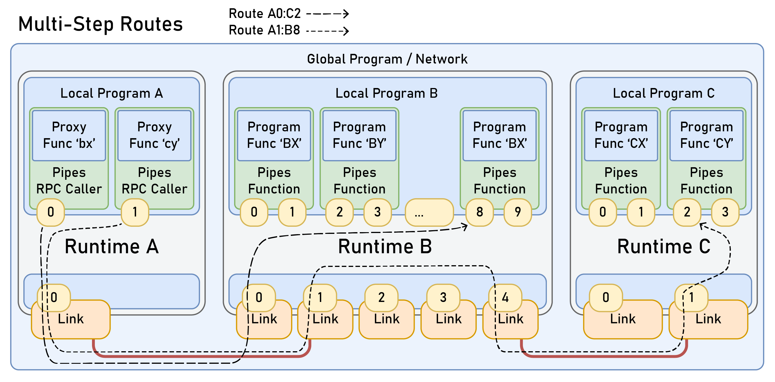
| Route | 1st Bytecode | 2nd Bytecode | 3rd Bytecode |
|---|---|---|---|
| A1:B8 | link_forward(0) |
port_handle(src: 0, dst: 8) |
|
| A0:C2 | link_forward(1) |
link_forward(4) |
port_handle(src: 1, dst: 2) |
| C2:A0’ | link_forward(1) |
link_forward(1) |
port_handle(src: 2, dst: 1) |
Routes can be extended across potentially many links by adding instructions, Figure 2.5 shows one example of this (it corresponds to Table 2.2). link_forward instructions are only one byte (encoding up to 64 ports per runtime, the first two bits contain the opcode and the last six are used for the opcode itself), the provision for bus_forward is two bytes (for 64 fieldbusses per runtime with 255 drops on each bus).
The port_handle opcode instructs the runtime that the packet should be delivered to a software module. It has two arguments: destination and source port indices. These are used by the runtime to deliver the packet to the appropriate port, that port also receives the source port and source route (which is reversed), both of which are required to generate a reply. This instruction is three bytes in length, source and destination indices are 11 bits each for a limit of 2048 unique ports per runtime.24
The final opcode is a system_message, at the moment those are used only for time synchronization (see Section 2.3.2.2), but up to 64 of these codes could be implemented for i.e. trace packets.25 There is allocation for a bus_forward opcode as well, with an argument for the bus gateway index and an additional argument for the network address on the bus of the receiving runtime. This is not implemented in the current version of OSAP but Section 2.9.1.1 discusses their inclusion, as fieldbusses are very common in industrial systems.
| Code Key | Bytes | Arg | Arg |
|---|---|---|---|
link_forward |
1 | Link Index [2:8] (64 Gateways) |
|
bus_forward |
2 | Bus Index [2:8] (64 Fieldbusses) |
Bus Drop [8:16] (255 Drops, 1 Broadcast) |
port_handle |
3 | Source Port [2:13] (2048 Ports) |
Destination Port [13:24] (2048) |
system_msg |
1 | Message Code [2:7] (64 Keys) |
[0:1] of any given code, and arguments are inserted piecewise into the succeeding bits, [inclusive, exclusive] and zero-indexed.
Packet headers contain two additional values, both of which are 16-bit. The first is the route’s Maximum Transmission Unit (MTU) which defines the underyling link layers’ largest data packet size in bytes. Where routes hop across multiple links, the smallest MTU of all links in the route is used. This is an important consideration because MTUs can vary widely in different link layers, for example CAN bus is often limited to 64 bytes only whereas Ethernet frames can be as large as 1500 bytes, some IP links allow up to a full 65 536 bytes per frame, and inter-process sockets in unix operating systems have variable underlying MTUs that are mostly based on buffer sizes. Encoding the MTU in every packet does consume considerable packet header space, but it ensures that low-level operation is stateless and the trade is that even very large MTUs can then be used whenever they are available, which improves efficiency.
The other header value is a time to live (TTL) stamp in microseconds, which is the basis for OSAP’s earliest deadline first scheduling - more discussion on that to come. A complete packet header that specifies one routing step (a link forward) between two ports in two different runtimes is shown in Table 2.4 below.
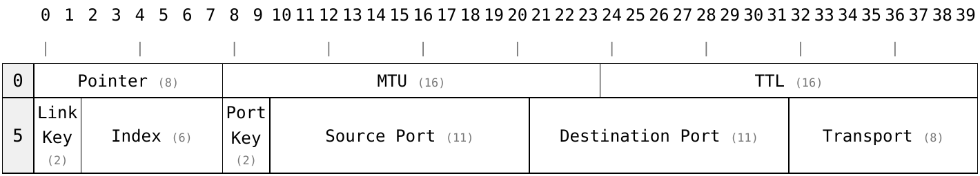
2.3.1.4 Memory Allocation and the Message Stack
The central data structure in the runtime is the “Virtual Packet,” see Listing 2.11 for the definition of the VPacket structure in the embedded runtime. These store raw packet data, the packet’s arrival time and service deadline, and pointers to the runtime component that owns them.
The stack is at the very core of OSAP’s runtime: service deadlines are used to schedule overall operation and packet allocation and deallocation is a key component of the flowcontrol system. Packets move between components in the runtime via pointer ownership, so they are also a kind of memory bus.
typedef struct VPacket {
  // data and it's size,
  uint8_t data[PCKT_MAX];
  size_t len = 0;

  // the scheduling deadline and time of arrival,
  uint32_t serviceDeadline = 0;
  uint32_t timeOfArrival = 0;

  // pointers to packet owners,
  // only one of which is valid at any given time
  VPort* vport = nullptr;
  LinkGateway* linkGateway = nullptr;
  OSAP_Runtime* runtime = nullptr;

  // for linked list operation,
  VPacket* next = nullptr;
  VPacket* previous = nullptr;
} VPacket;
In workstation scale computing the depth of this stack is virtually unlimited relative to the average packet size but on embedded devices allocating memory manually requires extreme care.26 Microcontroller memories are also limited and so robust embedded designs prefer static allocation. I use static allocation of packets in both cases (Python and embedded) to match operation throughout but in embedded the scheme is slightly more involved, as I will explain.
// in `packets.h`
boolean claimPacketCheck(VPort* port); // check if a stack slot is available,
VPacket* claimPacketFromStack(VPort* port); // claim a packet,
void relinquishPacketToStack(VPacket* pck); // release the packet
Ports and link gateways may try to generate new packets at any time and write them into this stack, but memory and CPU time is limited. To allocate access to the stack fairly, each port and link can only own a finite number of stack slots at any given time. This limit is configurable on a per-port and per-link level, i.e. you can see in the link gateway (Listing 2.8) and port (2.7) a maxPacketHold value. When implementing simple link layers that do not contain their own internal buffers - or very small ones - the stack can effectively extend these buffers.
In Python it is easy to expand the stack size such that all ports or link gateways can be “full” at any given time, but in embedded devices we sometimes need to limit stack use globally as well as on a per-component basis. There, each component uses the functions in Listing 2.12 to check for, claim, and relinquish stack space.
2.3.1.5 Flow Control
Flow control is a common problem in networking. We have the fundamental problem that data sources will often want to produce data at a rate that data sinks cannot manage. This takes form in a few different ways, the first of which was just mentioned: memory is not unlimited and so packets cannot be written by ports or pushed from links into the runtime when the stack is completely allocated. On the other side, ports need time to handle data and links are not always “clear to send” new data: their transmit buffers may still be full with prior data or their downstream partners may be equally busy. This extends end-to-end in the case where very fast devices transmit very many packets that must be consumed and processed by very small devices.
OSAP manages flow control on these two ends (sources and sinks): the stack interface controls flow into the stack as I described above, and messages will not be cleared from the stack before links or ports that will handle them are busy. You can see the software interfaces for this in Listing 2.8 and 2.7 (clearToSend, clearToReceive). The runtime’s main loop routine in Listing 2.13 also reflects this operation. Application layer flowcontrol is additionally performed at the transport layer, as is done in IP networks.
2.3.1.6 Scheduling and QoS via Earliest Deadline
Flow control and scheduling are related because both are related to how we operate networks under resource constraints: limited bandwidth and limited CPU time. I covered a broader background on networking constraints that includes some discussion of scheduling in Section 2.2.2.1.
As I’ve mentioned, operation in OSAP is scheduled around packets’ service deadlines: packets that are due to expire soonest are handled first, using the “earliest deadline” method that I have already mentioned which is based on [29] who note that this method out performs priority-based scheduling under heterogeneous loading scenarios.
Deadlines are calculated based on their arrival time within the runtime (which is also stored) and their packet-encoded time-to-live. Rather than sorting the packets according to this value in each runtime loop, packets can be inserted into the stack (a linked list) based on their deadline so that in the next loop cycle new packets are already sorted into the order in which they should be processed.
Time-to-live is also the main software handle for configuring network Quality of Service (QoS) and is first written into packets at their source ports: for example Pipes Functions (2.4.2) expose this value for individual connections. Tighter deadlines will cause packets to be serviced earlier than others, so they are a proxy for network priority and also encode - well - deadlines: if we have a control loop that must happen within a certain interval, we can transmit its data with a time-to-live that corresponds.27
When a link gateway transmits a packet it updates the time-to-live encoded in the packet header (see Section 2.3.1.3 for a table of packet encodings) according to the transmitting runtime’s measurement of that deadline, i.e. removing the interval of time that has elapsed28 since the packet was written into that runtime. This way the time-to-live value decreases as the packet traverses the network and overall timing can be maintained. At the moment this does not account for the wire time (the interval that the packet spends actually being transmitted) which can be substantial. Future work could use coordination between the synchronization service and this layer to ameliorate this. This type of interaction is one of the many ways that network layers - while we may try to separate them - remain intimately related to one another.
2.3.1.7 OSAP’s Main Loop
Considering each of these steps, we can now see how the runtime’s main loop runs - the core routine contains these four steps:
- Run
loopfunctions defined by each port and link gateway. - Traverse the message stack, which is sorted against packet deadlines:
- De-allocate packets whose deadline has passed.
- For packets addressed to Ports, reverse the route (2.3.1.3) and the source port index, and call the receiving Port’s
onPacketfunction if it isclearToReceive,de-allocate the packet if so, or continue (leaving it on the stack for the next cycle). - For packets that should be forwarded through the network, read the next routing instruction, and forward it via the link’s
sendfunction if it isclearToSend,deallocate the packet if so, or continue. - Handle
system_msgpackets.
- Run the time synchronization routine from Section 2.3.2.2; send clock queries to neighboring devices if the control interval has elapsed.
This tight loop is run repeatedly and so blocking code at any of these steps can cause e.g. a number of packet deadlines to expire at once. This amounts to cooperative scheduling, which is a common strategy for simpler runtimes like OSAP’s. In Section 2.8.3, I discuss how OSAP is likely to require preemptive scheduling (where ongoing tasks can be interrupted by the main loop) if it is to become a truly robust system. The cooperative strategy is exceptionally simple and does not lead to major issues if code is designed appropriately.
2.3.1.8 Transport
Software can be implemented directly on top of ports, which would be equivalent to the use of UDP packets in IP-based networks. However, we can also insert software-defined transport protocols. These are implemented between software (which may want e.g. delivery guarantees, timing guarantees, sequence guarantees, or to frame large messages over a series of packets) and ports (which are stateless). The first byte in any port-to-port message’s data frame is a transport_key, which ID’s the type of transport layer that the message is sent by. This is a provision to deconflict transport layers, so that messages that are improperly addressed can be handled appropriately.
So far I have only authored two of these: a very simple Sequential Transmitter and Receiver that provide order-of-delivery guarantees and allow us to easily reply to a particular message (not just a particular port) which helps software to ensure that responses to particular RPC (Remote Procedure Calls) (Section 2.4.4.2) are resolved against the correct call.
Transport layers in network systems are some of the most complex, and can introduce large overhead. The internet has annealed around TCP (Transport Control Protocol) but it is rarely used in networked control because of this overhead and state: messages can end up trapped in queues for long periods, etc. Transport control protocols are in fact controllers, i.e. the work that I discussed earlier in the background section on network design itself as an optimization problem made reference to Chiang’s work [46], where transport control itself is considered as a distributed control problem across many layers.
In this work, streams of data basically fall into two categories: configuration steps which can be slow but can fail if delivery guarantees are not provided, and operation where missing a packet is permissible and transport control is not strictly necessary. This is typical of networked controllers, and is another reason that we want to have flexibility in this layer as well.
2.3.2 OSAP Services
2.3.2.1 Network Discovery
I mentioned in the background section on source routing 2.2.2.2 that the main drawback to the strategy is that it becomes difficult to configure routes themselves, because this must be done manually. This is OK in static systems like SpaceWire [117] because i.e. the James Webb Space Telescope’s physical network configuration does not change very often and so routes can simply be written offline against system schematics and loaded into firmwares. For a reconfigurable, modular system it is obviously an issue.
So! OSAP also includes a kind of “distributed DNS” layer to allow discovery of network topologies. This effectively follows the Model-View Controller (MVC) architecture that I discussed in Section 2.2.3.5.
OSAP Runtimes each implement a “netresponder” class on their 0th port, which corresponds to the controller in the MVC framing. These reply to queries made by “netrunner” instances in other devices, which are responsible for ascertaining global network state - the view. The runtime’s internal structure is the model, in this case the total view spans multiple runtimes and involves also using information in source routes themselves to ascertain the structure of the network that connects them.
Each query and response uses data serializations that are pre-determined and written at a low level. While it would be possible to implement these using Pipes Functions (since they are basically RPCs), that would collapse the network and application layers and so goes against the design ethos of the stack. These are the queries:
- Get Runtime Information
- Get Runtime Type Name
- Get Runtime Name
- Set Runtime Name
- Get Link Information
- Get Port Information
- Get Debug Messages
- Set Debug Verbosity
- Get Time Controller Configuration
- Set Time Controller Configuration
To collect network state, the netrunner code does a breadth-first search over runtimes. It begins by querying its own runtime to ascertain how many link gateways it contains and whether or not they are open, and then writes a packet to traverse each of those gateways and query the runtimes connected to each, etc. Source routes are useful again here because they can be built sequentially in each recursion of the traverse and because they themselves represent network topologies.
OSAP allows that there can be multiple paths to the same devices, which may be beneficial in control systems where we would want to send data on one link and receive it on another, or otherwise use i.e. multiple routes between two devices to increase overall throughput and reduce latency, perhaps sending traffic that requires determinism over one link and burst traffic over another. This means that networks can contain loops and a simple recursive breadth-first search would go on endlessly if they were not de-conflicted. To do so, the Get Runtime Information message cycles an incrementing UUID (unique to the scan) that is transmitted by the netrunner and stored by the netresponder, which replies with the UUID from the last time it received one of these messages. If the netrunner sees a UUID that it previously generated in another lookup, it knows that the device is connected in a loop - and it knows which device this is, to map that loop to the network map.
Operationally, addresses in OSAP are all based on source routes (which are sometimes called “network addresses”). Those are relative, not global; in Figure 2.5 the network address of runtime C from the viewpoint of runtime A is different from the network address of runtime C from the runtime B. This in itself is not an issue when we are configuring a system from one viewpoint, but OSAP implements an additional human-readable naming scheme specifically because it is invaluable at the next layer up, when we start to write programs on these networks - which is what networks are normally made for in any case. The internet’s DNS is the same: to visit a website one does not type in the IP address of its web server.
I mentioned in Section 2.3.1.1 that runtimes themselves each have name, type name, version, and build fields. The names are just strings, the version field is three bytes (so version numbers can span 0.0.0 - 255.255.255), and the build field is keyed - it encodes whether the runtime is an embedded / C++ system or a Python runtime (etc).
Ports and link gateways each have name and type name fields as well. Their names can be semantically meaningful but are most often left blank, because the type name is what tells software (like PIPES) that i.e. this port contains a Pipes Function, which will contain its own semantically meaningful data when queried.
I originally designed OSAP itself to be completely nameless in the spirit of layer separation in the OSI model, but leaving “hooks” into the next layer at the edges of other layers is invaluable. The discovery of complete distributed programs would be infeasible without these names. In Section 2.8.4 I expand on this theme and reflect on some larger discourse around protocol design between the OSI model and the TCP/IP stack.
2.3.2.2 Distributed Time Synchronization
OSAP provides a clock synchronization service, which is used as a basis for motion control and for time series data collection. Since other clock sync algorithms are complex and consume large amounts of program memory, I developed a simple version that is loosely based on well understood principles from the well established Network Time Protocol (NTP, [30]) and Precision Time Protocol [10], but also on [31], where diffusion is used as a basis for synchronization.
System time is measured in microseconds using uint64_t to eliminate overflows. Runtimes request timestamps from neighboring devices at some configured interval (I use \(50ms\) in most networks), inserting their own timestamp at the head of the packet when they do so. When the neighbor receives that packet, they add a timestamp of their own system clock estimate and their clock tier and then return the packet. Using these data, the runtime calculates its offset to the neighboring clock and runs a simple PI29 controller to adjust its own clock skew, shimming it up to catch up to neighbors or down if it is overrunning. This is described in Listing 2.15. Parameters for the clock’s PI controller and the offset estimation filter are tune-able via the netrunner / netresponder interface.
- On a configured interval, transmit timestamp query packets to the runtime’s nearest neighbors over any open link gateway. Insert the runtime’s own time estimate into the packet’s first eight bytes.
- If a timestamp query is received, insert the local timestamp in the succeeding eight bytes and the local clock tier in the final byte, reverse the route and send the packet to its transmitter.
- When a reply is received:
- Calculate the query’s round trip time (RTT) using the timestamp made at packet generation and the current time and then estimate the (N) neighbor’s current system time using \(t_{\text{N,now}} = t_{\text{N,stamp}} + \frac{1}{2}\text{RTT}\).
- Measure the offset between the local system time and the neighbor’s system time.
- Apply an exponential weighted average to the offset estimate and store that for each neighbor, along with its clock tier.
- Select the best neighboring clock:
- Pick the clock with the highest tier.
- Update our tier to be that clock’s tier plus one.
- If multiple neighbors have the same tier, compute the average of our offset estimations to each.
- Using the computed offset estimate to the best neighboring clock as an error signal, apply PI control to the local clock.
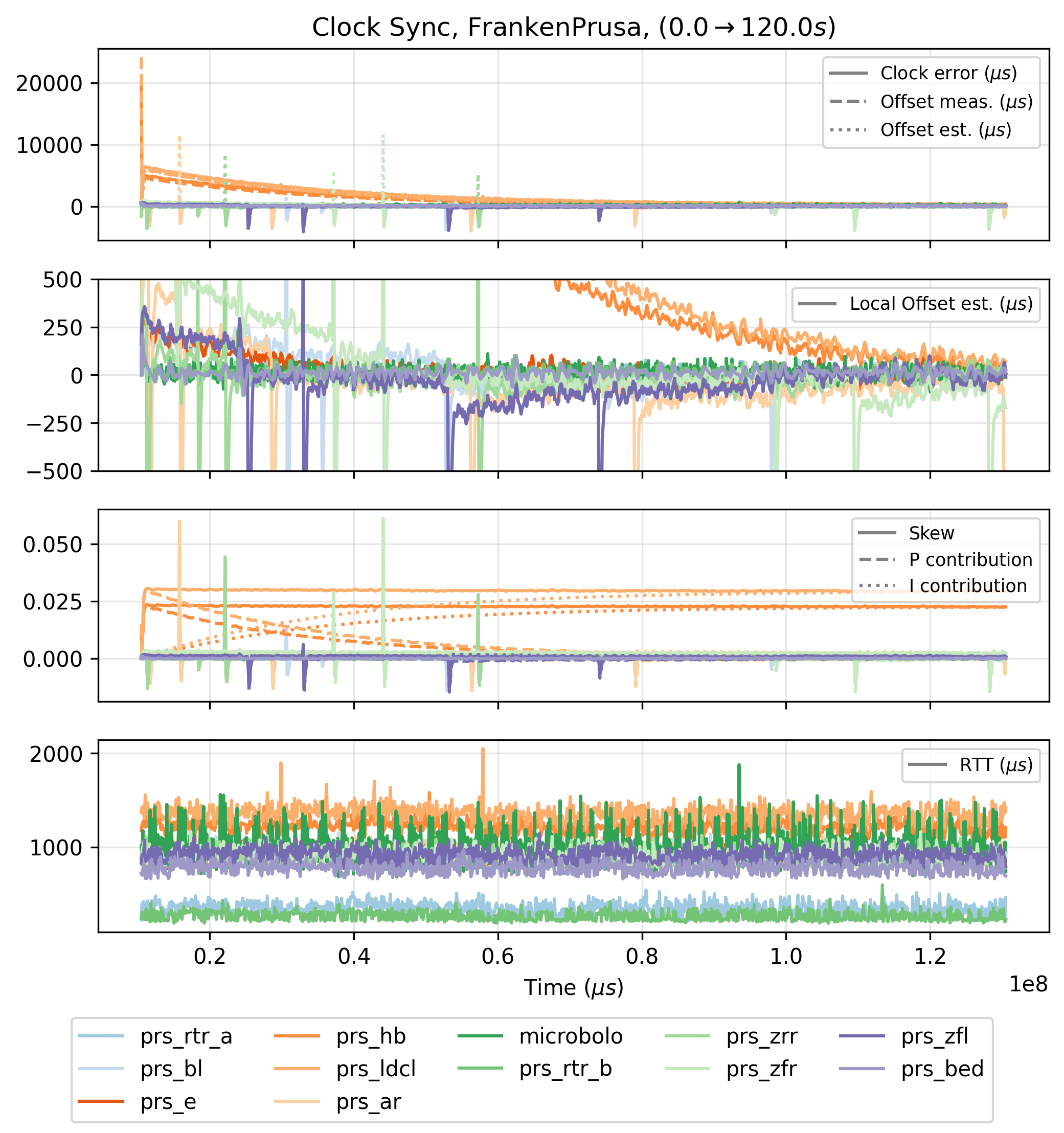
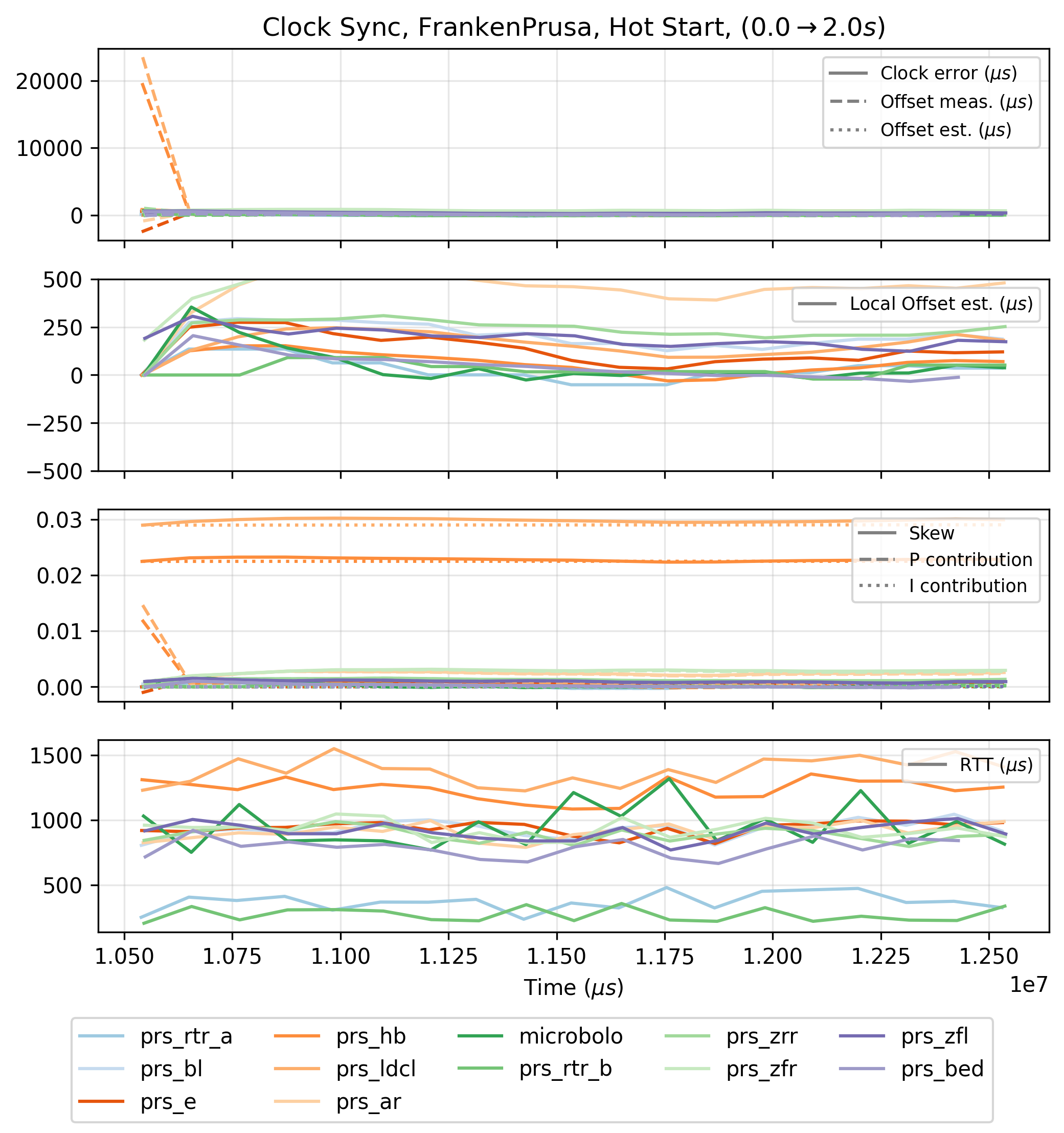
In the test above, we can see that clocks adjust to within \(500\mu\mathrm{s}\) with one another after \(60s\) and within \(250\mu\mathrm{s}\) after \(100s.\) Devices running faster microcontrollers tend to have better sync performance. Two caveats, the first being the rather obvious disturbances on these plots, where it seems that the controllers are being kicked out of band momentarily - I discuss this in Section 2.9.1.3. The second is that \(60s\) is a long time to wait for acceptable clock synchronization. To ameliorate this, we can hot start the synchronization controller, by storing clock skews after longer time synchronization runs and re-loading them into firmware when the system is initialized.
Time synchronization data also provides a quick proxy for network latency, in Section 2.7.9 I use some of these data for a simple evaluation of OSAP’s own performance.
Overall, the synchronization in OSAP works well enough for me to complete all the tasks in this thesis. It is clearly not perfect, and high performance synchronization is a requirement of advanced control systems. I discuss future work on the topic in Section 2.9.1.3 and address those errors below.
2.3.2.2.1 Time Synchronization Errors
Before carrying on here, I would like to discuss the periodic errors in the clock synchronization test, shown in Figure 2.6 and also seen in the test data in Figure 2.7 below.
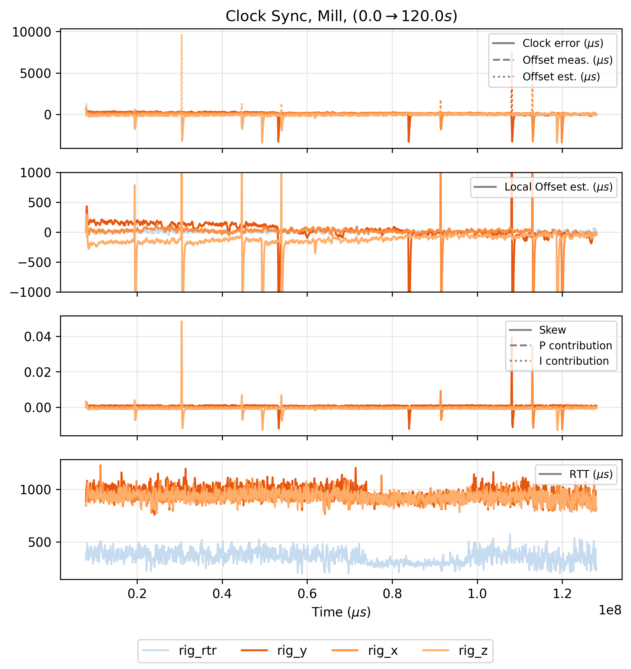
These spikes are not perceptible in any data sets that I saw prior to running these tests, and don’t cause any audible or visual disturbances while machines are running, but they are clearly problematic. We can see that they only appear on the motor drivers. This is more clear in Figure 2.7, where the Knuckles hub (3.5) device (labelled rig_rtr here), is in blue and the motors are in red / orange hues.
The motor controllers use many control interrupts, which can get preempt the clock synchronization routine. It seems likely that that is causing this issue, via a race condition or by causing asymmetries in the round-trip time measurements (where e.g. one leg of the transmission takes longer than the other, because the \(\mu\mathrm{c}\) is busy processing non-network tasks).
Luckily the clock controller recovers from these disturbances quickly, but this reveals is a clear example of the type of issue that emerges due to OSAP’s cooperative scheduling, and of the scheduling problem more generally. To work well the timing system may need to preempt the controller, but who is to say which takes precedence?
2.4 PIPES: a Programming Model for Partitioned Systems
Programming In Piped EcoSystems
PIPES runs on top of OSAP and is responsible for naming and describing software objects, building and modifying systems representations, configuring data flows between objects, and remotely calling software objects. PIPES uses a dataflow programming model to configure and represent controllers, but also mixes in scripting tools that make the tasking problem easier. PIPES’ configuration tools are presented as a software API, so that scripts which run machines can sequentially configure them programmatically, and then run those configurations — i.e. get them up and running.
In this section I first discuss the core design principle in Section 2.4.1, which is to source data schemas from devices and then apply programs on top of those schemas. This is in contrast to most other distributed systems programming tools where systems-wide schemas are first developed and then components are each written against those schemas. I then cover how functions (their source code directly) are used as a source of those schemas, and are wrapped in a network interface that embeds them as dataflow blocks and as Remote Procedure Call (RPC) implementations (Section 2.4.2). This wrapper includes a small Model-View Controller (MVC) that allows us to extend OSAP’s network discovery service from Section 2.3.2.1 to develop a programming model that combines dataflow with scripting, in Section 2.4.4. Programmer’s interactions here are mediated by a Manager software object, which produces proxies (2.4.4.2) and allows remote configuration of dataflow connections (2.4.4.3), all of which are represented by the underlying Systems Object Model (the SOM, 2.4.4.1). For all of these steps I developed a standalone serialization and typing scheme that is described in Section 2.4.3.
2.4.1 Runtimes are Schema Sources, not Sinks
In Section 2.2.3 I surveyed a selection of state-of-the-art distributed programming systems. Each of those uses an Interface Description Language (IDL) as a shared representation of how system components should interact with the system; IDLs are written by hand and they are the surface against which systems integrators and component developers work.
For example to integrate a new module or program with one of these systems, a programmer writes their device’s internal program, imports the IDL, and then authors “glue code” that connects their program to the IDL, defining new functions to call when certain data are received, and which functions will deliver data to certain topics (which are labelled), at which intervals and under which QoS parameters.
PIPES takes a different approach, which is to allow each device to describe its own interface and then expose those in a way that is discoverable so that global maps of devices and their interfaces can be discovered. In Section 2.4.4.1 I describe how that process works; we build a Systems Object Model which effectively replaces the IDL on a per-system basis. For a more in-depth comparison see Section 2.6.1.1 and Figure 2.25 in Section 2.6.1.2.
PIPES_FUNC macro to generate interfaces.
// in knuckles_loadcell `main.cpp`
float _lower_thresh = 0.0F;
float _upper_thresh = 0.0F;

// normally used as an RPC,
void setupComparator(float lower_threshold, float upper_threshold){
  _lower_thresh = lower_threshold;
  _upper_thresh = upper_threshold;
}

// normally configured to transmit at an interval through a Pipe
// returns a timestamp *and* the comparator's output value for
// resynchronization with other motion control states upstream
auto getComparatorReading(void){
  auto [time, reading] = getCalibratedReading();
  if(_lower_thresh < reading && reading < _upper_thresh){
    return std::make_tuple(time, true);
  } else {
    return std::make_tuple(time, false);
  }
}

PIPES_FUNC( // the Pipes Function wrapper generator, a C++ template
  setupComparator, // a reference to the implementation,
  "lower_threshold, upper_threshold", // provided argument names,
  "" // names for return values (empty)
);

PIPES_FUNC(
  getComparatorReading,
  "", // no input arguments
  "time, in_bounds" // output value names,
);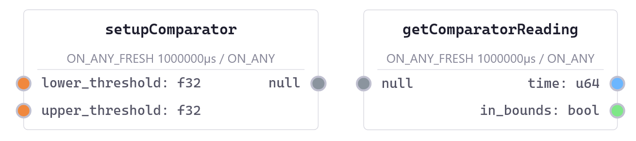
PIPES_FUNC in Listing 2.16 are wrapped by PIPES and source their data schema and network interactions, to produce systems-wide programming models.
This could involve writing a smaller interface within each device and then collecting each of them piecewise into a larger, global IDL. This is what MQTT [61], MSGFlo [84], and some other embedded bridges into distributed systems do; XRCE-DDS [65], Micro-ROS [66], and [67], [68].
In PIPES the approach is to use function definitions directly, rolling those up into interfaces by way of modern programming patterns like template programming in C++ and function “decorators” in Python. These are “code introspection” tools that allow programs to analyze themselves, and the insight is that programming languages’ own internal typing and naming schemes are descriptive enough to be used as interface descriptors directly. I cover some more background on this type of strategy (and how my use of it differs from the state-of-the-art) in Section 2.6.1.1.
The major benefit to this strategy is that it means that the schema we use to assemble systems has been built from a “single source of truth,” which is the schema’s implementation itself. Here, we extend that to mean not only that schemas are consistent, but that their representation as functions is consistent. In applying the same operational scheme across these functions, we can make sense of systems-wide operation by way of coordinating networks of functions.
The tool that I use for this is the PIPES_FUNC compiler macro in C++ and the @pipes_function decorator in Python. Both of them ingest function implementations and produce what I call Pipes Functions, both using interface classes that mediate between the implementation and the system, which I will describe below.
2.4.2 Functions as the Basic Building Block
Using functions directly allows module developers to reflect their native program representations directly to systems programmers, but it requires that we develop a network interface that wraps functions, attaches them to OSAP networks (on top of ports), and mediates between serialized network data and their actual implementations. This happens in two steps: first we build a state machine around the function (Figure 2.9) that will call the native function (the implementation) according to system-defined rules and based on network flows and messages, and then we build a controller for that state machine that can be queried remotely to generate a remote view of its configuration — another piecewise MVC layer (Section 2.4.2.6).
I call these interfaces Pipes Functions, in a sense they are like the Link Gateways from OSAP: they mediate between programmer-defined implementations (of functions themselves or of link drivers) and systems-defined operation of the same.
2.4.2.1 A State Machine to Embed Pipes Functions in PIPES Systems
The key figure here is 2.9, which describes the state machine and MVC that wraps each function implementation. I will describe each part of this figure in more detail in the next subsections, but for a quick map: we have the actual implementation at the core in orange, and see that runtime-native code can still call this function directly - so can other functions within a class instance (in the case where the function is a member of that class). The green blocks are inputs and outputs to the function - these are captured as the function’s argument list and return values. Items in blue are network configuration and discovery handles, and yellow blocks represent various network transactions: the RPC call and interactions with other Pipes Functions as dataflow components (see Sections 2.4.2.3 and 2.4.2.4). Grey blocks represent external data sources and sinks.
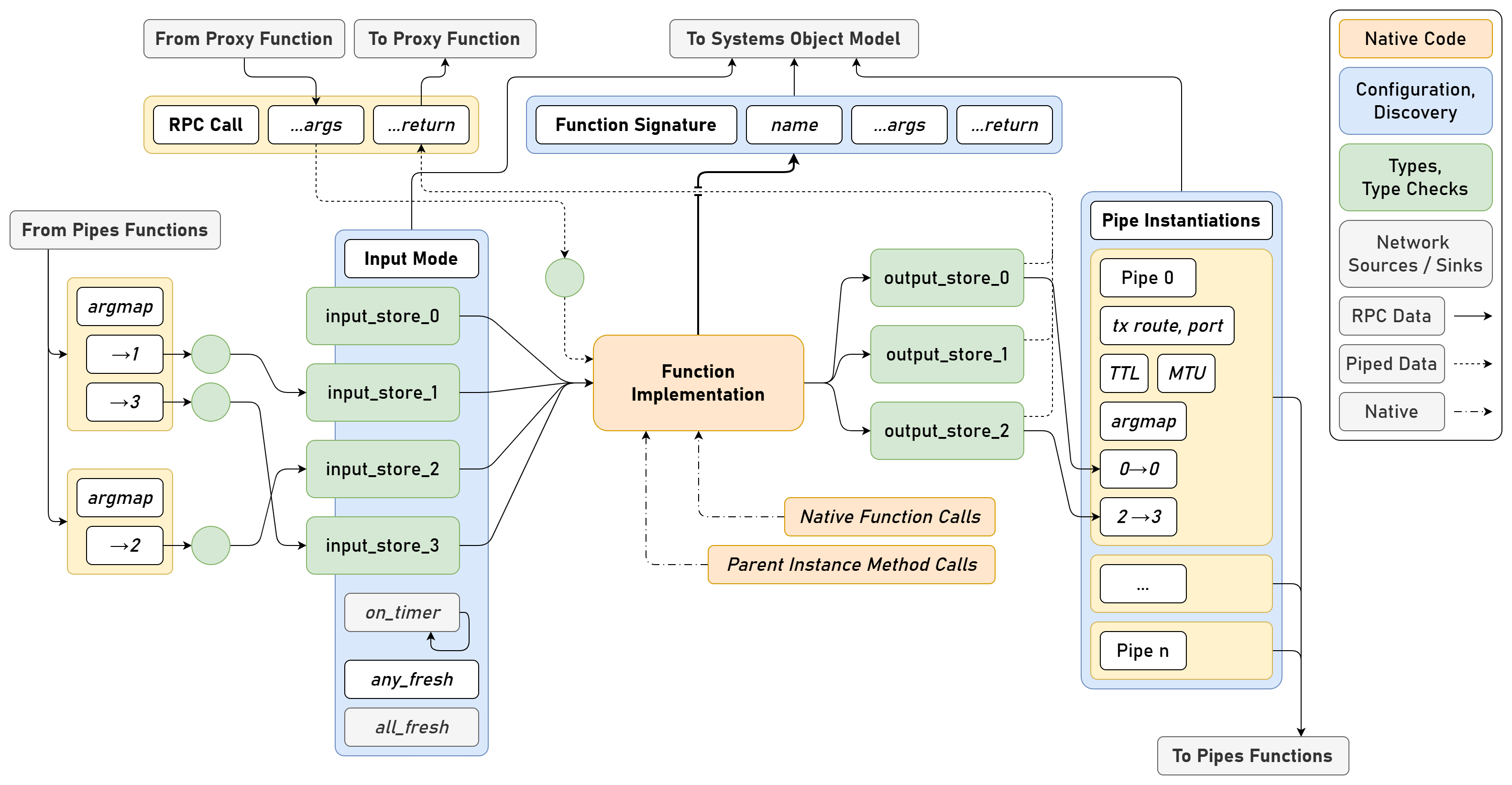
2.4.2.2 The Function Signature
A function’s “signature” is just its native interface: the function’s human-readable name, the names of its arguments (and their types) and their output type. In many cases functions only return one value (or none), but in some languages and practices returning tuples (typed lists) is common. I found this to be an invaluable design pattern in PIPES and MAXL, as will become clear. Those are also typed, but it is not common for values returned by a function to have names; implicitly the function name itself is equivalent to the return value name. I added some tooling that allows function authors to specify what names should be applied to tuples, which you can see in Listing 2.16.
The function signatures for our two loadcell functions are in the listing below alongside serialized configuration values for their input mode - this is how they appear in a serialized Systems Object Model. You will see that these also include a “localPort” value, which maps the function to the OSAP port where it is attached.
setupComparator from Listing 2.16.
{
  "name": "setupComparator",
  "inputs": [
    {
      "name": "lower_threshold",
      "typeName": "f32",
    },
    {
      "name": "upper_threshold",
      "typeName": "f32",
    }
  ],
  "outputs": [
    {
      "name": "",
      "typeName": "null",
    }
  ],
  "inputMode": "ON_ANY_FRESH",
  "inputInterval": 1000000,
  "localPort": 4
},getComparatorReading from Listing 2.16.
{
  "name": "getComparatorReading",
  "inputs": [
    {
      "name": "",
      "typeName": "null",
      "value": null
    }
  ],
  "outputs": [
    {
      "name": "time",
      "typeName": "u64",
      "value": null
    },
    {
      "name": "in_bounds",
      "typeName": "bool",
      "value": null
    }
  ],
  "inputMode": "ON_ANY_FRESH",
  "inputInterval": 1000000,
  "localPort": 5
}
Not any function can be rolled up as a Pipes Function. Input and output types must be atomic values in the core PIPES type set (which includes most ANSI C types (plus strings), see Section 2.4.3), and there are practical limits to the length of type names and type values that are not clearly articulated to programmers; for example this architectural stack does not yet implement the transmission of multi-packet datagrams, so it is implicit that serialized data structures need to fit within a single packet.
It is also the case that Python functions are not always strictly typed, and so Pipes Functions can only be applied to functions that implement complete type hints, a somewhat recent syntax addition to Python.
2.4.2.3 Interactions with Remote Procedure Calls
Remote Procedure Calls (RPCs) are a common design pattern in distributed systems ([59] Section 4.2). They are atomic operations (one request, one response) and simply mirror the function call in a remote device. In Figure 2.9 the RPC is in the top-left, and data flows in that case are represented with a dashed line.
The RPC call packet is generated by a function proxy (see Section 2.4.4.2) and contains a message type key (denoting that it is a function call), and the input arguments that are serialized against the function signature. Serialized argument types are checked against the local signature and conversions are applied if they are available (again see the Pipes Types section 2.4.3), and then serializes the return values and replies to the caller.
So far this is just a classic RPC implementation, but in PIPES there is the added side-effect that the RPC call’s operation of the implementation generates new output values (green blocks to the right of the implementation in 2.9). If Pipes (see the next section) have been instantiated on this function, those new values will be transmitted according to their configurations.
2.4.2.4 Function Interactions with Dataflow Graphs
To Pipes Functions we can attach Pipes, the atomic object (not the system itself PIPES). In Figure 2.9, these are diagrammed in a column (blue border, yellow Pipes) to the right of the function’s output values.
A Pipe is a dataflow connection that collapses network and program operation. We can attach any number of Pipes to a function, but are again limited in embedded systems by memory (and everywhere by compute and network bandwidth) requirements for these objects.30
Each Pipe instantiates a new OSAP Port so that messages can be generated in parallel for each pipe and so that transport flow-control from one does not impede the other (etc). Each has a configuration, which is below:
- A transmit route and port that specifies how the data should be routed through the OSAP network, and to which Pipes Function port. This is configured against the Systems Object Model, and also includes the route’s Maximum Transmission Unit (MTU, see Section 2.3.1.3).
- An argmap that specifies which function outputs should be transmitted to which of the recipient’s inputs. This amounts to two lists:
- A list of Output Arguments i.e.
0, 2in the first Pipes instance shown in Figure 2.9. - A list of Input Arguments i.e.
0, 3.
- A list of Output Arguments i.e.
Configuring Pipes such that they can “weave” output and input indices together in this manner was another key design pattern that I developed alongside MAXL, for example in Figure 2.10 below, where one example of this pattern is shown (and explained in the figure caption).
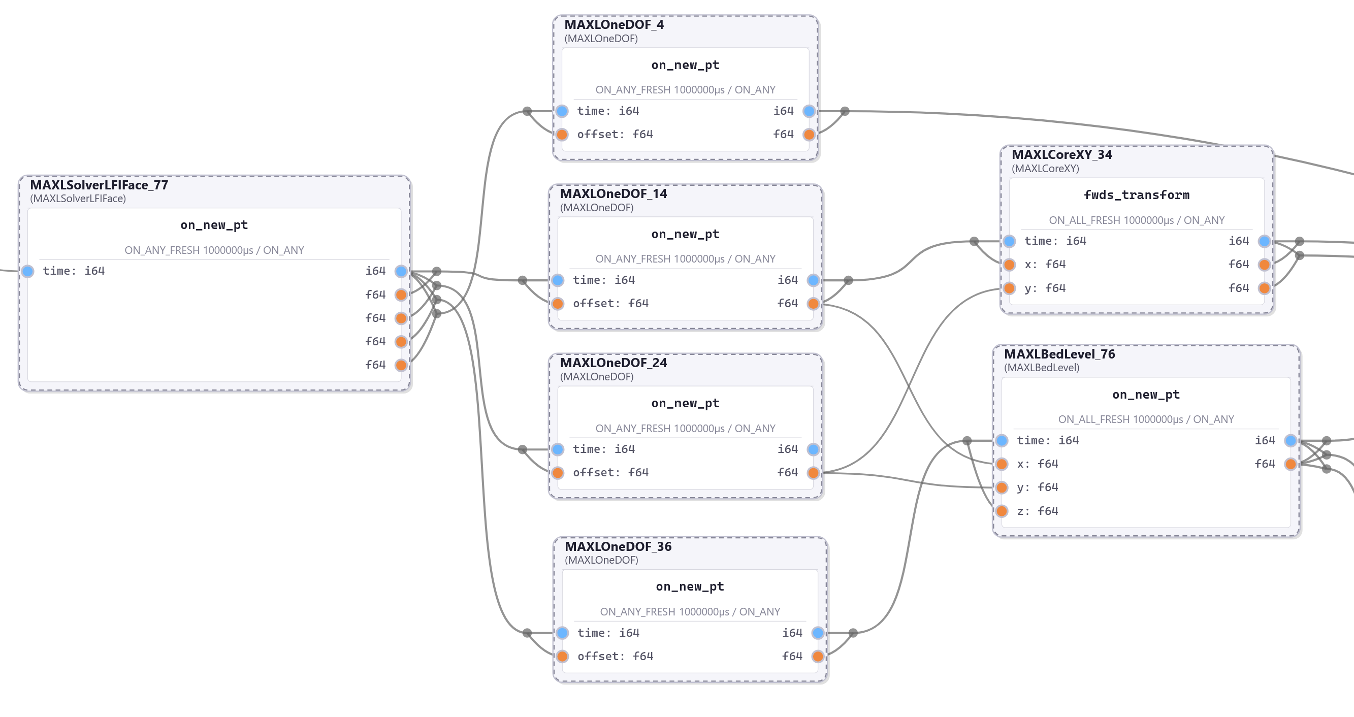
argmap configurations. In this example a motion control planner’s output from on_new_pt (at left) is a tuple of (time, x, y, z, e) control points. That is mapped into a series of OneDOF MAXL blocks (see Section 2.5.4.2), each of which is applied to one axis only: the maps are e.g. (0, 1) -> (0, 1) for the second OneDOF (in x) and (0, 3) -> (0, 1) for the third OneDOF (the z axis).
Pipes are responsible for serializing outputs, and do so whenever new outputs are available and their downstream transport layers are clear and a new packet can be allocated, if not they wait until these conditions are met. However they do not contain internal buffers and so when i.e. two new outputs are generated during an interval when the Pipe has been awaiting clearance to send data downstream, one of those outputs is missed.31
Woven inputs are applied to Pipes Functions at the left-hand side of Figure 2.9. When a Pipes Function receives data from another function, it deserializes these values and loads them into the input stores here, marking them as “fresh,” meaning that they contain new data. They are additionally type checked / converted at this point if the configuration and types allow it.
The input mode configuration defines when the function will be called according to these values’ freshness. I have developed three modes, on_any_fresh and on_all_fresh, which are explained by their names: one is used to eagerly call the function on any new data and the other is used to wait for each to be updated before operating the function. In dataflow programming models this is known as “input resynchronization.”32
It is worth noting that in this scheme we can easily write Pipes that transmit to other functions in the same runtime, or even that transmit data from the function back to itself. This is because PIPES is based on a networking model, not on direct graph analysis and execution as is the case in some other dataflow programming models like Grasshopper [118], where entire graphs are analyzed before they are run and loops cause infinite analysis cycles.
2.4.2.5 Functions as Class Members
I extended the PIPES system to include classes as groups of functions, but only completed this exercise in Python where code introspection is more straightforward.33
This has the main purpose of allowing us to deploy groups of functions that can change one another’s output via the classes’ internal state. Class functions can call one another in their local scope, and can update states that affect functions which are part of dataflows.
This side-effect means that we can operate dataflow objects via function calls, and this is a key capability for the merging of dataflow with scripting that PIPES implements. The MAXL design pattern emerged on this basis: each MAXL block is a Pipes Class that has a core function that samples timestamps (and other streamed control points), and then operates on those to generate new outputs. Other methods in the same class are used to update that core function’s behaviour according to the current task being performed by a global control script.
Pipes Classes extend the Pipes Function; the constructor’s function signature is captured in the same manner, and the Pipes Class MVC is extended such that we can recover which Pipes Functions are bundled within that class. Functions within classes can be marked with a leading underscore to indicate that they should not be included in the Pipes Class.
Finally, Pipes Classes can each implement a loop function; PIPES will call this function once on each cycle of its OSAP runtime loop. This can be used by the class to generate periodic outputs according to its own internal logic.
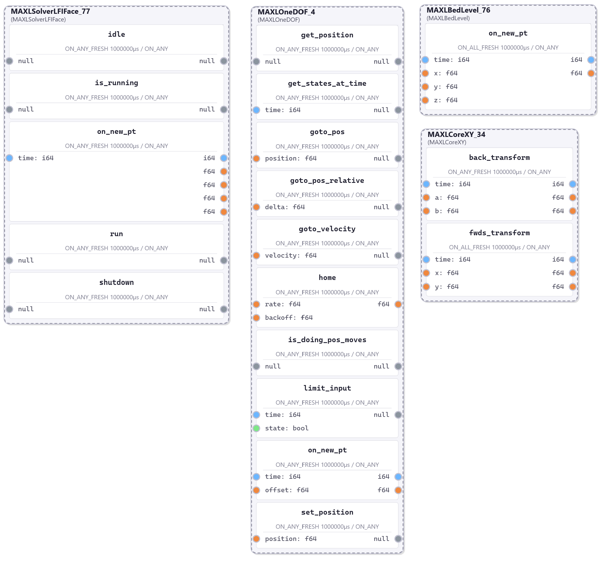
@pipes_class_implementer
class MAXLOneDOF:
    def __init__(self, max_vel: float, max_accel: float, output_scalar: float):
        self.max_vel = max_vel
        self.max_accel = max_accel
        self.output_scalar = output_scalar
        self.output_offset = 0.0
        # delta-tee tracker
        self.most_recent_timestamp = -1
        # states tracker
        self.position = 0.0
        self.velocity = 0.0
        self.velocity_target = 0.0
        # for offsets
        self._pos_offset = 0.0
        # stores latest limit states
        self.limit_time = 0
        self.limit_state = False
        # stores pts for history lookup, and blocks for motion
        self.control_points: Deque[MAXLOneDOFControlPoint] = deque(maxlen = 4096)
        self.segments: List[MAXLQueueSegment]
2.4.2.6 The Function’s Model-View Controller
I have discussed the Model-View Controller (MVC) design pattern in a few places: an overview of the pattern and my implementation of a kind of network MVC in OSAP (Sections Section 2.2.3.5, 2.3.2.1).
Each Pipes Function also implements an MVC: the model being the function and the Pipes state machine (which encompasses the function signature, its input mode configuration and its output Pipe instantiations), the controller being a part of the network wrapper for that function, and the view being a piecewise component of the larger Systems Object Model.
This pattern appeared in OSAP as well: each component (in that case the OSAP runtime) contains its own small MVC, and we run a larger cycle over a collection of these to create a global view at the systems level.
While we add a new OSAP port for each configured Pipe, each Pipes Function is initialized with just one port, and messages to that port are switched according to a pre-determined key code; this includes messages that
- Get Function Signature
- Remote Procedure Call
- Pipe Datagram (as a Dataflow Component)
- Get Pipe Count (Dataflow Output Wires)
- Get Pipe (retrieve one Pipe configuration)
- Set Pipe (add one Pipe configuration)
- Wipe Pipe (remove one Pipe Configuration)
- Get Input Mode
- Set Input Mode
It is perhaps worth noting that a Pipes Function’s output configurations (to wire data to other Pipes Functions) is useless without the surrounding network map and definitions of the recipient functions, this is the property of source routed networks that I have discussed in a few places. In Section 2.4.4.1, I will explain how we use a global search to do systems-scale reconciliation of these piecewise descriptions.
2.4.3 Types and Serialization
PIPES uses a core and internally consistent serialization scheme that is based on the ANSI C set of datatypes; each type gets a systems-wide keycode which is used in the leading byte of every serialized value and also to serialize function signatures.
Listing 2.22 shows these keycodes, each PIPES system includes these in their source files - Quentin Bolsée and I designed this together in an attempt to make it extensible across compounding types, for example the bitmask of the Array type can be or’d with other key bitmasks to produce a compound. Table 2.5 shows how a Pipe is serialized, this matches the Pipe configuration that is rendered in Figure 2.9.
// are names and bitwise representations.
#define TYPEKEY_NULL    0   // null   0b00000000
#define TYPEKEY_BOOL    1   // bool   0b00000001
#define TYPEKEY_UNKNWN  3   // unknwn 0b00000011

#define TYPEKEY_I8      16  // i8     0b00010000
#define TYPEKEY_I16     17  // i16    0b00010001
#define TYPEKEY_I32     18  // i32    0b00010010
#define TYPEKEY_I64     19  // i64    0b00010011
#define TYPEKEY_I128    20  // i128   0b00010100

#define TYPEKEY_U8      24  // u8     0b00011000
#define TYPEKEY_U16     25  // u16    0b00011001
#define TYPEKEY_U32     26  // u32    0b00011010
#define TYPEKEY_U64     27  // u64    0b00011011
#define TYPEKEY_U128    28  // u128   0b00011100

#define TYPEKEY_F16     33  // f16    0b00100001
#define TYPEKEY_F32     34  // f32    0b00100010
#define TYPEKEY_F64     35  // f64    0b00100011
#define TYPEKEY_F128    36  // f128   0b00100100

#define TYPEKEY_ASCII   48  // ascii  0b00110000
#define TYPEKEY_UTF8    49  // utf8   0b00110001

#define TYPEKEY_ARRY    64  // arry   0b01000000
#define TYPEKEY_TNSR    128 // tnsr   0b10000000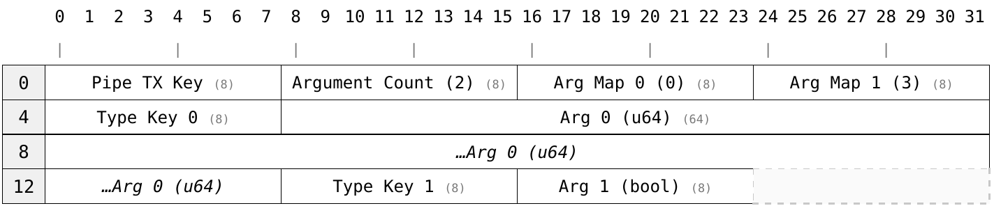
getComparatorReading defined in Listing 2.16.
PIPES’ serialization scheme is again designed to be more stateless than other schemes. It does so at the cost of packet size: each data stream contains full-width data and also type keys — where we are transmitting hundreds of thousands of these Pipes, adding a full byte per data object is hardly efficient. However, it avoids the state that would be required to establish stream type definitions ahead of their operation.
2.4.4 PIPES’ Systems Programmer’s Model: Scripted Dataflow
Configuring and tasking PIPES systems is done with two interfaces to one underlying representation, which is the Systems Object Model (SOM). Configuration and tasking is done only in Python at the moment, but it should be possible to develop similar design patterns in embedded devices. The complexity in these steps is much deeper though, and in many cases we prefer to run configuration and tasking steps from a more easily edited and more inspectable language like Python.
I developed a MetaManager class (it first appeared in Listing 2.6) to collect and manage the SOM. It is attached to an OSAP port in the host runtime and available there as a software object. In collecting the SOM from devices, we are essentially sourcing the system’s modular data schema from all the system participants themselves, and then using that unique SOM to program against.
The primary programming interfaces are remote procedure calls to Pipes Functions — which is done using proxies that are written based on the SOM (in Section 2.4.4.2) — and the manager.connect() function, which wires Pipes Functions together (see Section 2.4.4.3).
We cannot remotely instantiate new Pipes Classes or Functions, instead they are manually instantiated in each runtime. This is a major limit to overall systems reconfigurability and prevents us from more completely modifying lower-level controllers — e.g. adding PID code modules to existing hardware, that run in hardware — which could be an invaluable capability. In my Masters’ thesis [113] I did develop a version where embedded classes and function could be instantiated (and deleted) remotely, and I cover some of the steps that would be required to recover this capability in Section 2.9 (on future work).
We can still instantiate Pipes Classes within the Python runtime where our configuration code and tasking script lives, and use the system to develop flows between those classes and remote runtimes. This is productive enough to accomplish the controls tasks in this thesis.
2.4.4.1 A Systems Object Model
The Systems Object Model is not unlike the browser’s DOM, it is a hierarchical list of objects of predictable types but with unique names and properties. Objects in the SOM are represented by their human-readable names, which are mapped to network addresses “under the hood” by the Manager but are still available on closer inspection of the structure.
- A list of OSAP Runtimes, within each:
- A list of Link Gateways,
- A list of Ports,
- A list of Pipes Functions that have been globally instantiated there,
- A list of Pipes Classes that have been instantiated there.
- A list of Links, each of which has:
- A source Runtime and Link Gateway,
- A destination Runtime and Link Gateway.
- A list of Pipes, each of which has:
- A source:
- Runtime,
- Function Name,
- Class Instance Name (if the function is a member of a class).
- A destination:
- Runtime,
- Function Name,
- Class Instance Name (if the function is a member of a class).
- Output and Input indices to map the source function’s return tuple items onto the destination function’s arguments (the
argmapfrom Listing 2.19)
- A source:
The SOM is extended on top of OSAP’s network map, which is also used as the basis for discovery of the current configuration. For example the network map contains runtimes, link gateways and links (which connect gateways), and ports - each port has a type name (see Section 2.3.2.1), in the case of Pipes Functions these are human-readable as "pipes_function_rx", and in the case of Pipes (which transmit dataflows), as "pipes_pipe_tx" etc. These handles are used to generate additional Pipes Function MVC requests on those ports, collecting the software map.
The SOM is a flattened representation of a graph that may have loops, which simplifies its representation and allows us to serialize it as a .json, which I tasked an LLM to render as a visualized graph in a browser-based tool, that program is what generated figures like 2.12 based on SOMs that were saved from some of the systems that I deployed. That figure renders the FrankenPrusa’s controller (from Section 5.4.2).
The flattened representation is also used by the Manager class for the slightly more difficult task of building network routes between two Pipes Functions, as I will describe in Section 2.4.4.3 and for writing proxies, which I will describe in Section 2.4.4.2.
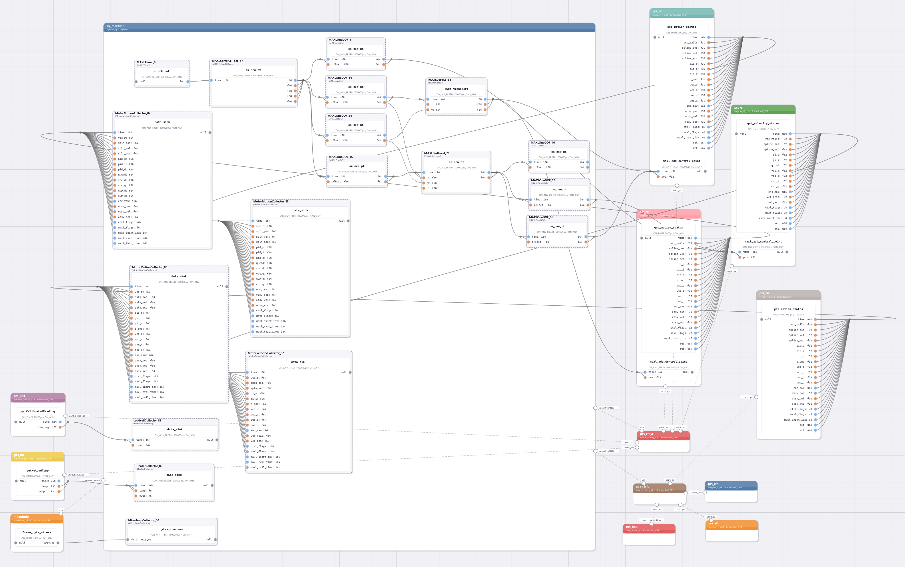
2.4.4.2 Proxies for Remote Components and RPCs
The SOM stores the underlying systems representation, but it is not very useful to directly program against. Instead we use proxies, following the Object Oriented Hardware pattern; they are software classes that can be instantiated in Python within one OSAP runtime, and that represent remote hardware: when we make function calls on these classes they operate that remote functions’ RPC and return the result. Like the PIPES manager, proxies are at the moment only developed for and deployed in Python.
I use the name proxy because I think that it more clearly articulates what the class is: an interface / stand-in object, rather than really “representing” the device itself. I used a templating language called Jinja [119] to write a “metaprogramming” tool that ingests the SOM and writes a series of .py files containing proxy definitions with one file and class definition per runtime / device, an example of which is in Listing 2.24.
Proxies provide a typed interface that can be called directly using RPC semantics or used as a handle to make connections, as I describe under the next header. Instantiating a proxy in your script implies to the manager that you expect that the device is present in the network at the time the script runs, when these instantiations are made the manager checks the proxy’s configuration against the most up-to-date SOM and if types or names are mismatched produces an error. This effectively prevents us from running systems against mistaken configurations.
Because systems themselves are mostly stateless before our configuration tool runs, we can run this process once whenever we have a new set of hardware configured, write the proxies, and then import those into a new script that we use as the basis for systems development.
class LoadcellCs5530D21:
    def __init__(self, manager: 'MetaManager', runtime_name: str):
        # a network-capable interface for each function definition
        # found in this device from the SOM,
        self._get_raw_loadcell_reading_proxy = PipesFunctionProxy(
            manager, # the system manager, which contains the loaded SOM
            runtime_name, # the system-unique runtime name to look for,
            "global", # class instance name, or 'global'
            "getRawLoadcellReading") # the function name
        # ...
        # ... omitting "_set_calibration_params_proxy"
        # ... omitting "_get_calibration_params_proxy"
        # ...
        self._setup_comparator_proxy = PipesFunctionProxy(
            manager, runtime_name, "global", "setupComparator")
        self._get_comparator_reading_proxy = PipesFunctionProxy(
            manager, runtime_name, "global", "getComparatorReading")

    # the programmer's interface is to these functions,
    # which are assigned type hints according to discovered function signatures
    # and adding """comments""" to roughly document the functions
    async def get_raw_loadcell_reading(
            self)-> Tuple[int, int] :
        """
        returns (time: int, reading: int)
        """
        time, reading = await self._get_raw_loadcell_reading_proxy()
        return cast(int, time), cast(int, reading)

    # ...
    # ... omitting "set_calibration_params" and "get_calibration_params"
    # ...

    # the "asyncio" interface releases the runtime while the network
    # retrieves the remote procedure call,
    async def setup_comparator(
            self, lower_threshold: float,  upper_threshold: float) -> None:
        await self._setup_comparator_proxy(lower_threshold, upper_threshold)
        return

    async def get_comparator_reading(self)-> Tuple[int, bool] :
        """
        returns (time: int, in_bounds: bool)
        """
        time, in_bounds = await self._get_comparator_reading_proxy()
        return cast(int, time), cast(bool, in_bounds)
2.4.4.3 Configuring Dataflows
To build Pipes Connections between functions, the manager implements a .connect() function. For arguments, it takes the proxies for the source and destination functions, and then argument lists (outputs, inputs) to map onto the pipe. For example Listing 2.25 writes the connections that result in the configuration shown in Figure 2.10 above.
When making these connections, the manager checks function signatures from the SOM to ensure that the connection’s output and input types either match or will be easily converted in hardware, and then finds the appropriate network route between the two devices (by traversing the SOM) and each function’s local port to complete the configuration. In .connect we can also specify the Pipe’s time-to-live as a network quality of service handle, to prioritize certain Pipes performance over others. Once the Pipe is in place, it updates the local SOM to reflect this.
Finally, proxies are also the handle through which we configure remote functions’ input modes, which I discussed in Section 2.4.2.4.
# maxl timer pushes events to the solver,
await manager.connect(machine.timer.clock_out, solver.on_new_pt)

# the solver transmits points from new solutions one-by-one to OneDOF blocks,
await manager.connect(solver.on_new_pt, machine.dof_x.on_new_pt, "0, 1", "0, 1")
await manager.connect(solver.on_new_pt, machine.dof_y.on_new_pt, "0, 2", "0, 1")
await manager.connect(solver.on_new_pt, machine.dof_z.on_new_pt, "0, 3", "0, 1")
await manager.connect(solver.on_new_pt, machine.dof_e.on_new_pt, "0, 4", "0, 1")

# leveler gets x, y states to evaluate the level correction at that position,
# and z, which it offsets using the correction,
self.leveler.on_new_pt.set_input_mode('all_fresh')
await self.manager.connect(self.dof_z.on_new_pt, self.leveler.on_new_pt, "0, 1", "0, 3")
await self.manager.connect(self.dof_x.on_new_pt, self.leveler.on_new_pt, "1", "1")
await self.manager.connect(self.dof_y.on_new_pt, self.leveler.on_new_pt, "1", "2")
# the leveler transmits updated z-targets to each z-motor's OneDOF block;
# instantiating one of these per motor is useful because each needs
# to be homed and offset independently of the others
await self.manager.connect(self.leveler.on_new_pt, self.dof_zfl.on_new_pt, "0, 1", "0, 1")
await self.manager.connect(self.leveler.on_new_pt, self.dof_zfr.on_new_pt, "0, 1", "0, 1")
await self.manager.connect(self.leveler.on_new_pt, self.dof_zrr.on_new_pt, "0, 1", "0, 1")

# corexy transforms the solver's XY outputs into AB values to suit
# the machine's kinematics
self.corexy.fwds_transform.set_input_mode('all_fresh')
await self.manager.connect(self.dof_x.on_new_pt, self.corexy.fwds_transform, "0, 1", "0, 1")
await self.manager.connect(self.dof_y.on_new_pt, self.corexy.fwds_transform, "1", "2")
2.5 MAXL: Motion Control with Dataflow
Modular Acceleration planning and eXecution Library
The development of MAXL is motivated by two main goals that I described earlier in Section 2.1.3.1. The first is to build motion controllers that expose a better software interface to their velocity planners. They are key machine control components that cause machines to accelerate and decelerate in order to smooth motion and avoid exceeding kinematic and actuator constraints (Sections 4.2.4 and 4.6 both describe this step in more detail). Trajectories encoded in GCodes cannot be interpolated in time because velocity planners live beneath the GCode interface. As I have discussed, this causes issues for machine builders and process researchers — the instructions that we send to the machine are modified, and we cannot ascertain what was actually done when our instructions (GCodes) ran. The second is to develop motion control as a system of modules that can be easily reconfigured for a variety of machines.
The challenge in this regard is threefold: first, we need synchronized execution of a planned trajectory in our distributed modules. The basis for synchronization in MAXL is OSAP’s clock sync service (Section 2.3.2.2), but we still need to write those trajectories and interpolate them. The second is to split operation of the controller across the realtime gap so that we can build smart controllers in high-level programming languages (which are not normally deterministic) but still smoothly run trajectories in embedded hardware, where we also do sensing of important machine states. Finally, we have the challenge of describing motion control in a modular fashion so that we can build controllers for a range of machines using a shared core of software components.
For these tasks I wrote MAXL (Modular Acceleration planning and eXecution Library); it develops motion controllers as dataflow graphs. We can then use PIPES configurations of MAXL blocks to combine kinematic transforms and corrections, look-ahead planners (4.2.4 and 4.6), and a host of other motion planning utilities (2.5.4) into new controllers.
2.5.1 MAXL’s Operating Principle
MAXL works by sequentially transmitting trajectory segments between dataflow blocks. Most of these blocks (Section 2.5.4) are written in Python as Pipes Classes, and trajectory interpolators are written in C++ as Pipes Functions. I originally developed the basic premise in [110]: by encoding trajectories as some set of functions that can be interpolated on a time basis, we can simplify trajectory execution so long as we have synchronized device clocks. To do so we broadcast trajectories throughout our system — ensuring that time-encoded segments arrive ahead of the time when they will be used — and then at any time, firmwares can query trajectories against their synchronized clock to pick an appropriate action. For closed-loop motors this means updating their position reference at some interval, and for steppers it means issuing a step signal whenever the interpolated value changes by more than one step, and so on. The scheme also makes the reconstruction of machine motion more straightforward computationally, because trajectories and sensor readings can all be reconciled as one time-series.

In that earlier paper, I developed a few types of interpolable functions: linear trapezoid segments to encode motion event tracks, which simply change value at set times and can be used as triggers for sensors or control set points for lower level systems. In this implementation I use only one: cubic basis splines (Section 2.5.3). I also extend the concept to use a dataflow configuration. The PIPES section already showed some examples of MAXL components, another is in Figure 2.14. This allows us to reconfigure motion control systems by re-wiring graph connections rather than re-writing software, and helps us to include motion control as a component of the larger distributed machine control system.
The premise in MAXL is that:
- Device clocks are synchronized.
- Timestamps tick along at a fixed interval, which is set by the Timer block 2.5.4.1. It outputs a new timestamp once in every interval.
- Other blocks (a set of which are explained in Section 2.5.4) can be combined using dataflow configurations to modify and generate motion control trajectories.
- Blocks trigger on these timestamps, using whichever logic they would like to implement to generate a new output value at that time, passing those through the dataflow chain alongside the original timestamp. In many cases, blocks add, multiply, or otherwise combine their contributions to that value with inputs that were generated by other blocks i.e. adding offsets or transforming from cartesian to actuator spaces.
- Any component can save local trajectory history, so that sensor readings and events collected later on can be compared with those histories.
- Besides operating or modifying these values, MAXL blocks can also interpolate them to produce reference signals that can be attached to hardware outputs (e.g. as position or velocity targets in a servo).
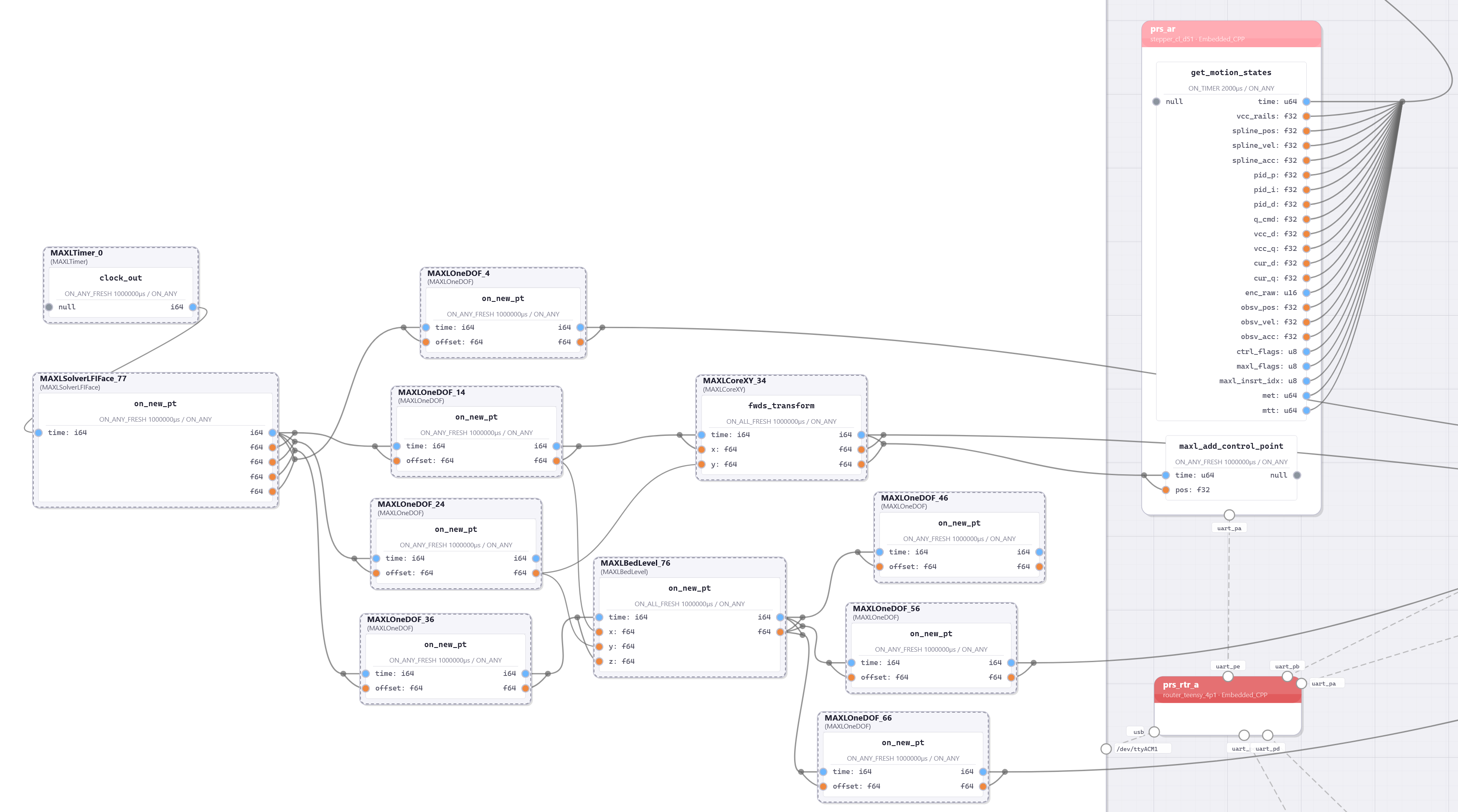
prs_rtr_a is a message passing device, dashed lines represent network segments.
2.5.2 The MAXL Gap
In MAXL, components are distributed across networks and some motion components are computed in non-deterministic languages and operating systems. This means that we need a strategy to ensure that the time gap between trajectory generation and interpolation is no shorter than the maximum interval that it may take for the trajectory point to reach the interpolator.
For simple linear segments this would mean that at any time interpolators have at least one control point in the future to interpolate towards. Basis splines require that they have two future control points in memory (and one in the past, see Section 2.5.3). At the same time, a smaller gap is better in many cases because it increases the high level bandwidth in our system.
So, in MAXL we configure a gap; the timer block generates a new timestamp whenever the current system time plus this gap exceeds the value of the last timestamp that it transmitted. The gap size can be configured against network and determinacy measurements such that it is minimized but is still larger than the minimally safe value.
In Figure 2.15 I diagram how this works; timestamp generation happens ahead of time and triggers blocks (in green) to compute new outputs. Those compute steps each add some delay, as do network segments in the graph. When the control points arrive at their interpolators they are stored in local queues where they are inserted with reference to their timestamp (so interpolators can also ascertain whether they have missed a point).
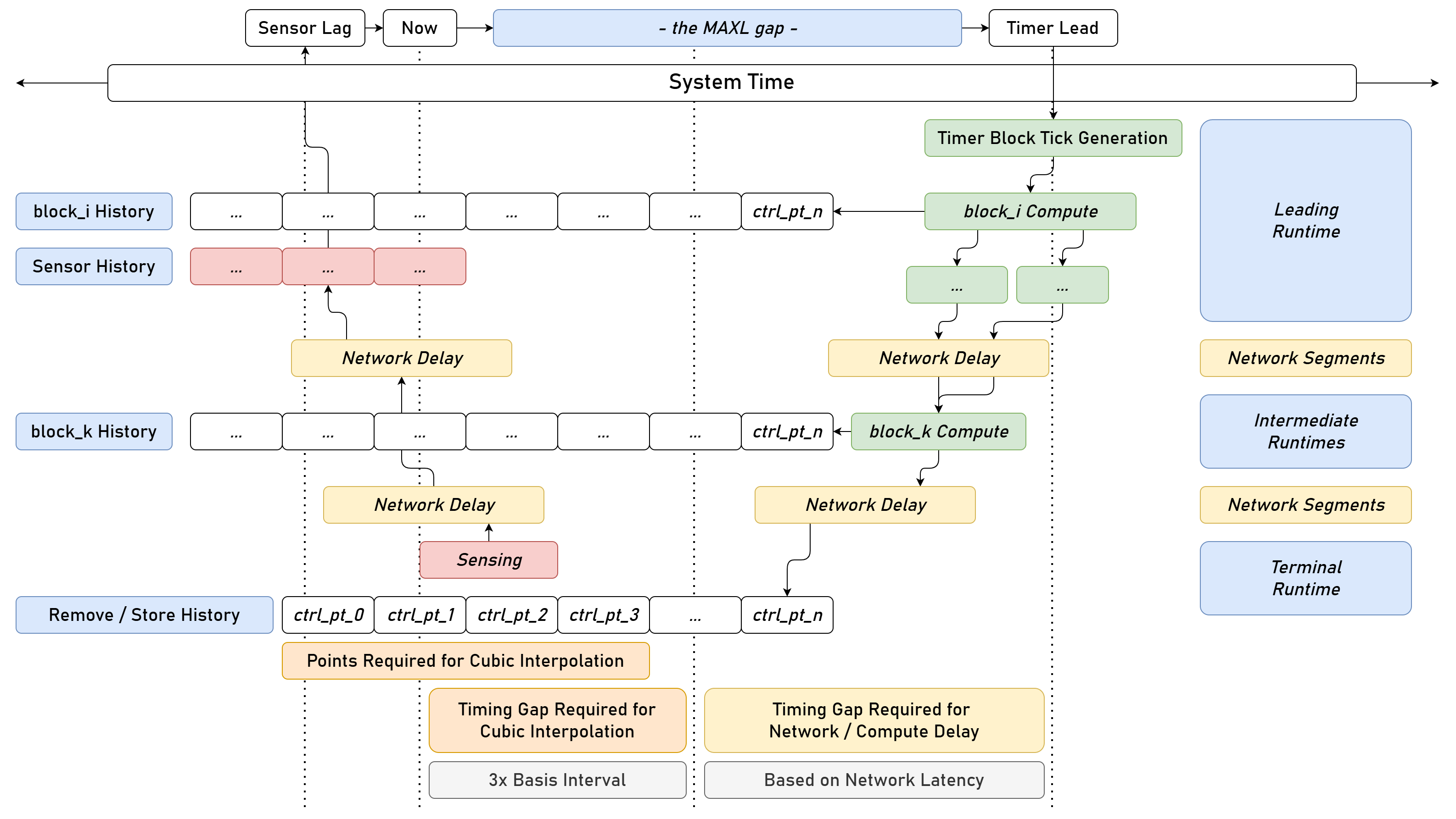
I have already mentioned why time-based encodings are valuable for the recreation of time series data and e.g. their combinations with sensor readings, but using a fixed interval also has some benefits. The first is straightforward; blocks that operate as integrators can then do so using a repeating \(\Delta t,\) which can simply them numerically.
The second has to do with network loading. Transmitting at a fixed interval makes for deterministic network loading; the amount of data that our network has to transmit in order to operate the controller does not change dramatically during the course of operation. We can compare this to spatial encodings that are used in GCode (line and arc segments), Klipper (small velocity-planned line segments) and i.e. StepDance and Urumbu (steps are small spatial deltas). Spatial encodings require that we transmit more data when we make faster or more complicated moves, and less at other times.
For example CNC milling machines often make long, linear traverses and then helical entries into the succeeding cut. The traverse is one line of GCode that takes a very long time, but the helix is composed of very many small linear segments (or small arcs) that each take a very short amount of time. This means two things: first is that the bandwidth requirement between the GCode “sender” and the interpreter can vary greatly over time (slow, and then fast very suddenly), and that the GCode interpreter itself must balance the two tasks (planning prior segments, running control outputs — and reading new GCodes, rebuilding them as internal representations, and adding them to the queue) simultaneously. These issues have largely been solved by modern interpreters by increasing their performance across the board, but some can still stutter under stresses like this. The underlying phenomenon means that we have to select queue sizes — memory buffers, not space or time — for our interpreters against these constraints: too long of a queue and our machine becomes unresponsive to new inputs, too small of a queue and the planner may be starved where geometries are dense.
2.5.3 Synchronized Basis Splines
To describe motion in time, MAXL uses a cubic basis spline interpolation (often just called a B-spline) with control points (aka knots) at fixed time intervals. Basis splines are commonly used to representation motion because they have well-defined and smooth definitions of velocity and acceleration with step functions in jerk [120]. This matches particularly well to inertial systems controlled by electric motors because they have the same order. I will discuss this in Section 4.3.1; our actuators cannot instantaneously change the amount of torque (acceleration) they are exerting, since it takes time for an applied voltage on the motor stator to develop into current. This means that electric motors cannot instantaneously change accelerations, although they can make instantaneous changes to the rate of change in acceleration (i.e. voltage, jerk).
I discuss how they contribute to the overall composability of MAXL in Section 2.8.2. Interestingly they also relate well to constraints-based optimization in both the network optimization sense and in the motion control sense, I discuss that coupling in Section 7.4. They do add a small amount of interpolation error because they are not direct interpolations, the interpolated path does not pass directly through their control points. I quantify this error in Section 7.4.1.
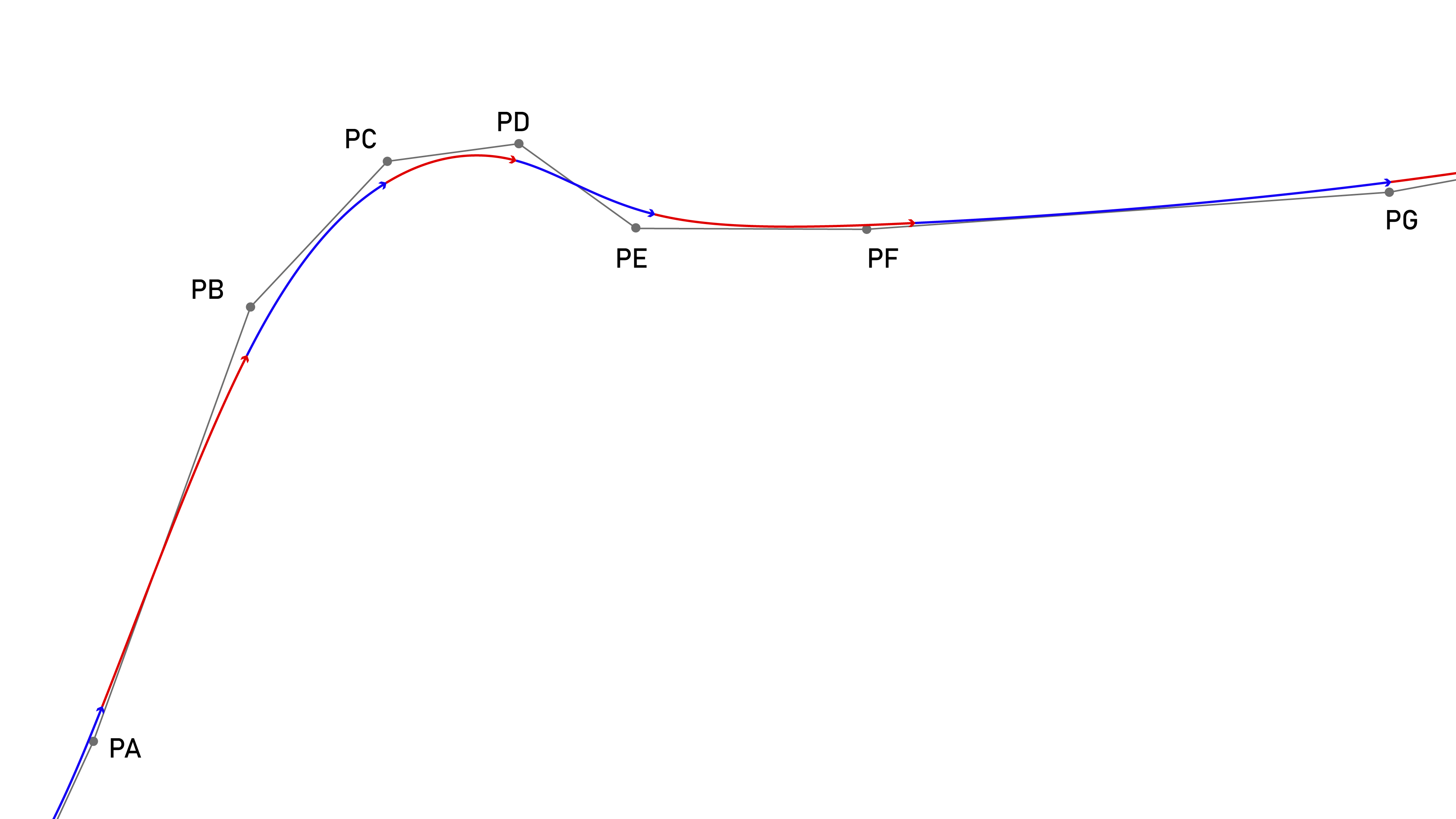
\[ \begin{bmatrix} P \\ V \\ A \\ J \end{bmatrix} (t) = \begin{bmatrix} 1 & t & t^2 & t^3 \\ 0 & 1 & 2t & 3t^2 \\ 0 & 0 & 2 & 6t \\ 0 & 0 & 0 & 6 \end{bmatrix} \frac{1}{6} \begin{bmatrix} 1 & 4 & 1 & 0 \\ -3 & 0 & 3 & 0 \\ 3 & -6 & 3 & 0 \\ -1 & 3 & -3 & 1 \end{bmatrix} \overbrace{ \begin{bmatrix} P0 \\ P1 \\ P2 \\ P3 \end{bmatrix} }^{A} \tag{2.1}\]
Equation 2.1 is the cubic basis-spline form that MAXL uses, which defines position, velocity, acceleration, and jerk (\(P,V,A,J \text{of} (t)\) — not all need to be evaluated) at any time based on the points in \(A\). Points in \(A\) can be vectors of any dimension; splines decompose well on a per-axis basis. The time \(t\) spans a fixed interval \((\Delta t)\), and the interval is set at some integer value of microseconds that is a power of two, between 256us and 16384us. Using these intervals means that the spline can more rapidly be evaluated using fixed point arithmetic in embedded devices. Basis splines have the helpful property that we can always add new points to the end of a stream, meaning that at each interval we only need to stream one new position whereas e.g. a velocity-planned linear segment of similar length would require much more information.
2.5.4 MAXL Blocks
MAXL Blocks are Pipes Classes that each perform a subset of the overall motion control and coordination task. I use them throughout this thesis to compose both complete motion systems and smaller controllers and calibrations. In these sections I provide a brief overview of how each functions and which roles they play.
2.5.4.1 Timer
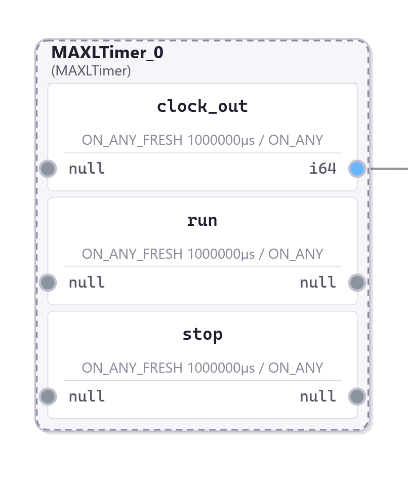
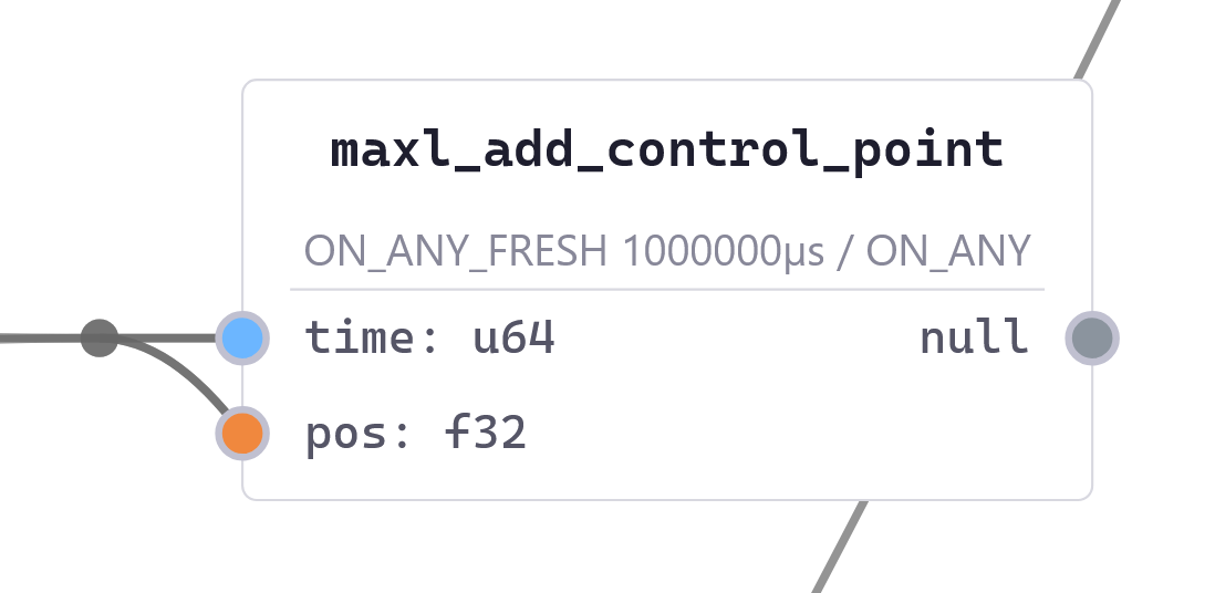
The timer block leads graph, generating one new timestamp within each interval. These ticks then flow through downstream blocks to produce new outputs.
We only have one timer block in any MAXL graph and it is configured with the system’s \(\Delta t\) and an advance parameter to span the appropriate gap (as in Section 2.5.2). For example if our interval is \(1024 \mu\mathrm{s}\) and advance=16, the timer will generate a timestamp for \(t = 16384 \mu\mathrm{s}\) at \(t=100000 \mu\mathrm{s}\), effectively leading the system clock by those \(16384 \mu\mathrm{s}\).
To decide if a new timestamp should be issued the block uses its loop function to evaluate OSAP system time against the defined gap size; if the current system time plus the gap is beyond the most recently transmitted timestamp, it generates a new one. This is rather than relying on i.e. a perfectly scheduled call to the timer output. If the runtime is temporarily blocked for more than one interval the timer will output a series of points in succession in order to catch up; the computation of the MAXL graph does not need to happen according to precise timings so long as smooth interpolation of the control points is maintained.
2.5.4.2 OneDOF
The OneDOF is a utility for controlling single degrees of freedom (DOFs). It is used in-line with axes of motion to add general purpose motion functionality to those axes. It contains a single-segment trapezoid generator that can be used to move DOFs smoothly from point to point and a velocity control mode that applies acceleration control, and is included in Figure 2.11.
This block also implements a simple homing routine where the limit switch signal is exposed as a Piped input, meaning that we can source home signals from any module in the system. For example to level 3D printer beds, I use a comparator output from the load cell sensor to trigger this “switch” in combination with a OneDOF block that is chained into all three z-motors.
2.5.4.3 Chirp Generator
The chirp generator is another simple motion utility that I use in the generation of preliminary motion models. It writes chirp time-series using scipy [121] and interpolates through them to produce outputs. These excite motion systems across a range of frequencies, which is useful for systems analysis.
2.5.4.4 Trapezoidal Planner
This is a classical type of velocity planner that I describe in Section 4.2.4. It ingests line segments, queues them, and does look-ahead velocity planning across them using direct parameters for a kinematic system’s per-axis maximum accelerations and velocities and a geometric parameter for deviation from path corners. I use MAXL and PIPES to virtually swap between this planning block and the model-based planner (block below) to compare the performance of this style velocity planner (which is the basis of most state-of-the-art motion controllers) with my model-based planner in Section 4.7.1.
2.5.4.5 Optimization-Based Planner Interface
The optimizers developed for velocity planning in this thesis are integrated within machine systems using MAXL via an interface block that I describe in Section 4.6.2.
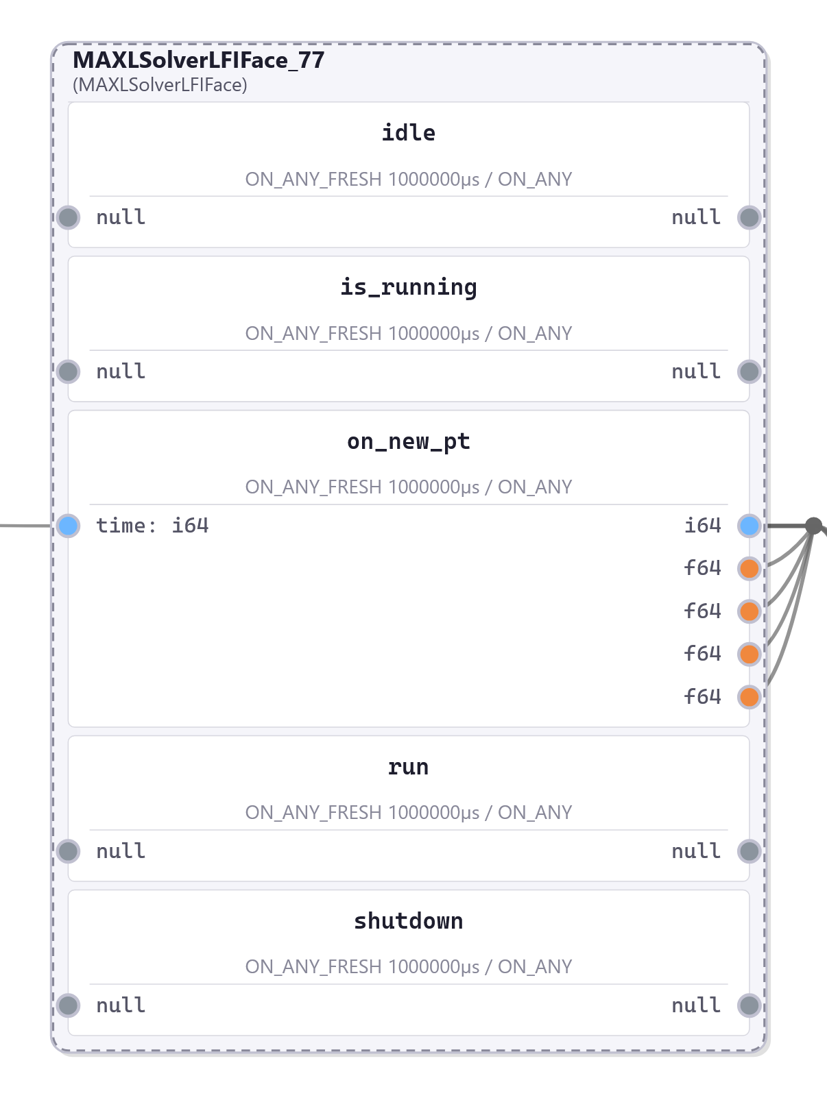
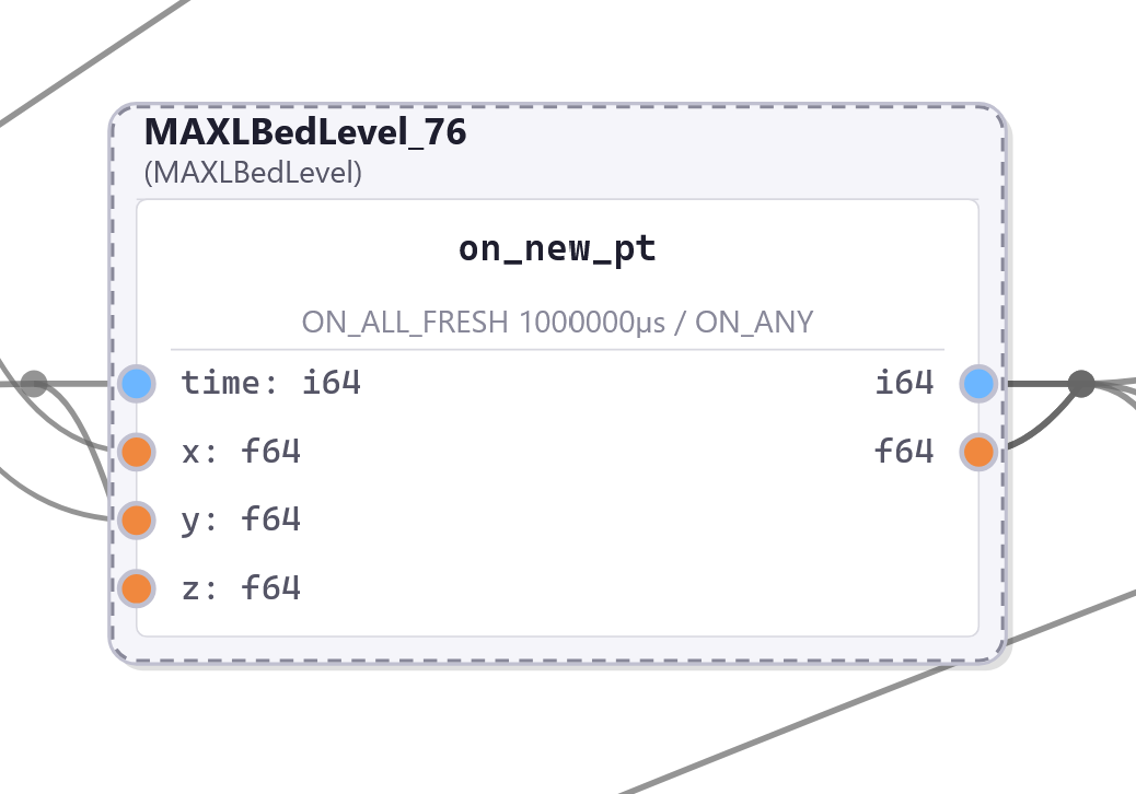
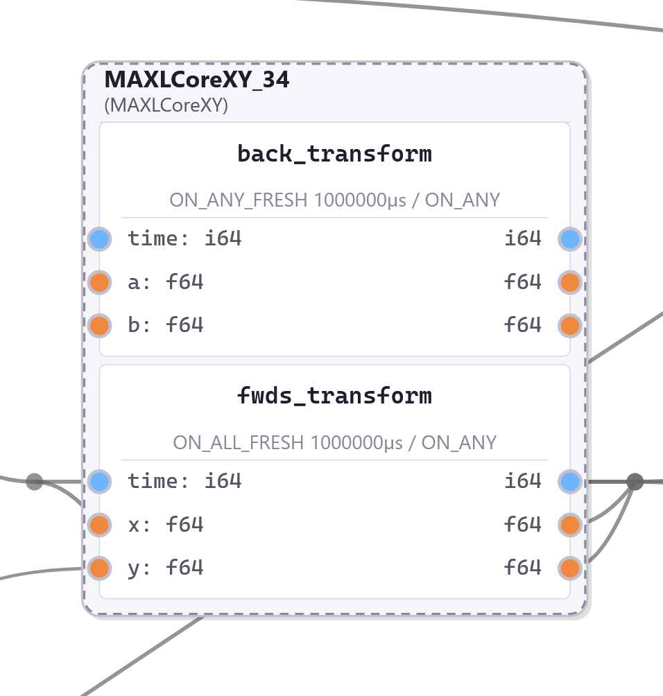
2.5.4.6 CoreXY Kinematics
This block implements CoreXY [122] kinematics and is used in both 3D printers that I developed (Section 5.4.1 and 5.4.2).
@pipes_class_implementer
class MAXLCoreXY:

    def fwds_transform(
            self, time: int,
            x: float, y: float) -> Tuple[int, float, float]:
        a = (x + y)
        b = (x - y)
        return time, a, b

    def back_transform(
            self, time: int,
            a: float, b: float) -> Tuple[int, float, float]:
        x = 0.5 * (a + b)
        y = 0.5 * (a - b)
return time, x, y 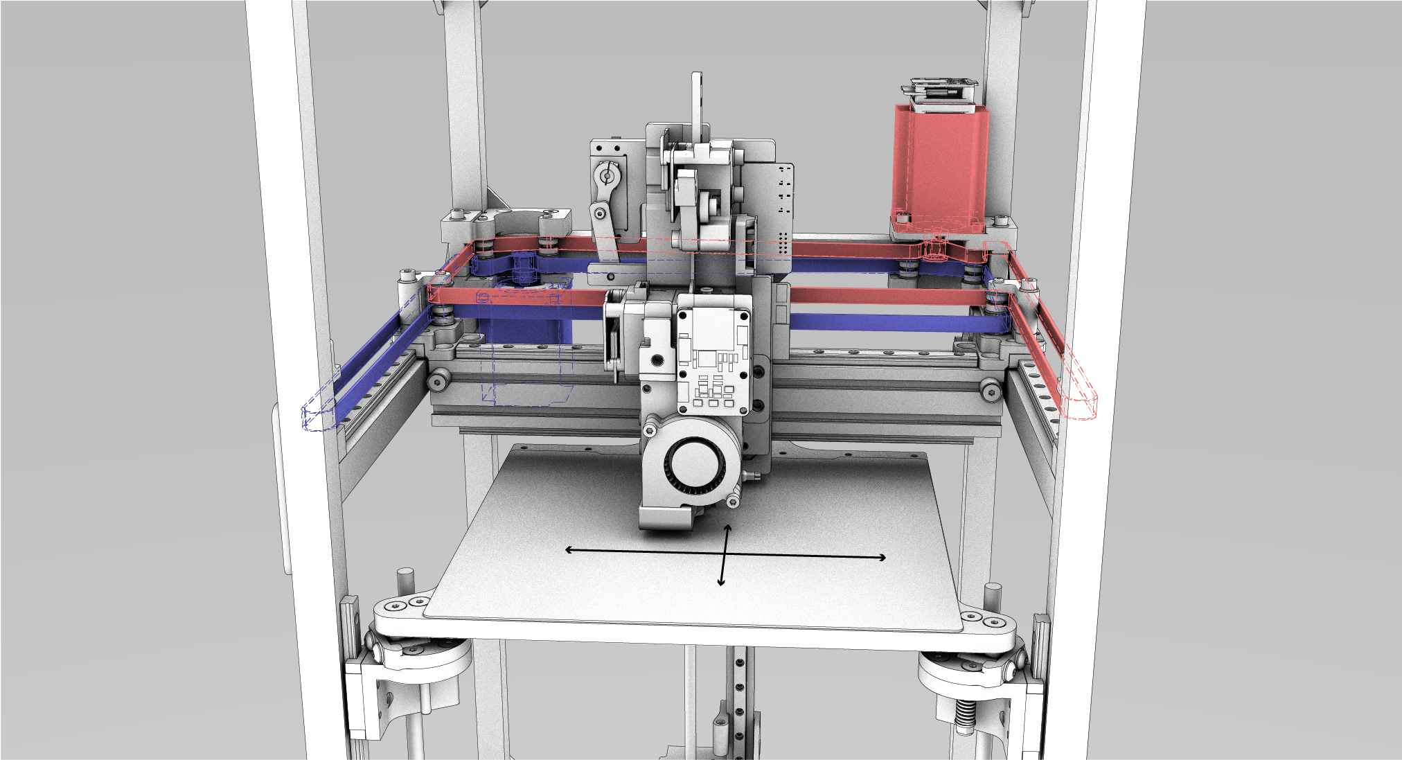
2.5.4.7 Scara and Kaos Kinematics
Both of these were developed in a machine building workshop that I discuss in Section 2.7.5.1, in an earlier version of MAXL and PIPES. The Kaos kinematics (Figure 2.23) require only a small update to the CoreXY function (for the angle of the V-shaped structure). The Scara kinematics (Figure 2.22) are nonlinear,
@pipes_class_implementer
class ScaraArm:
    def __init__(self, len_a_shoulder, len_b_distal):
        self.len_a_shoulder = len_a_shoulder
        self.len_b_distal = len_b_distal
        self.p_base = [0,0]

    # returns actuator angles *in degrees* and intermediate values,
    def cart_to_actu(self, time: int,
            x: float, y: float
            ) -> Tuple[int, float, float, float, float]:
        # the elbow is located based on circle-to-circle intersection,
        inter_a, inter_b = intersect_circles(
            self.p_base[0], self.p_base[1], self.len_a_shoulder,
            x, y, self.len_b_distal
        )
        # ad hoc guard for out-of-bounds values
        if inter_a is None or inter_b is None:
            raise ValueError(F"Singularity @ ({x:.2f}, {y:.2f})")
        # for elbow position, pick the biggest y always,
        p_elbow = inter_a if inter_a[1] > inter_b[1] else inter_b
        # some trigonometry,
        cos_shoulder = (p_elbow[0] - self.p_base[0]) / self.len_a_shoulder
        ang_shoulder = np.rad2deg(np.arccos(cos_shoulder))
        ang_elbow = 360 - np.rad2deg(
            np.arccos((x - p_elbow[0]) / self.len_b_distal)
        )

        return time, ang_shoulder, ang_elbow, p_elbow, cos_shoulder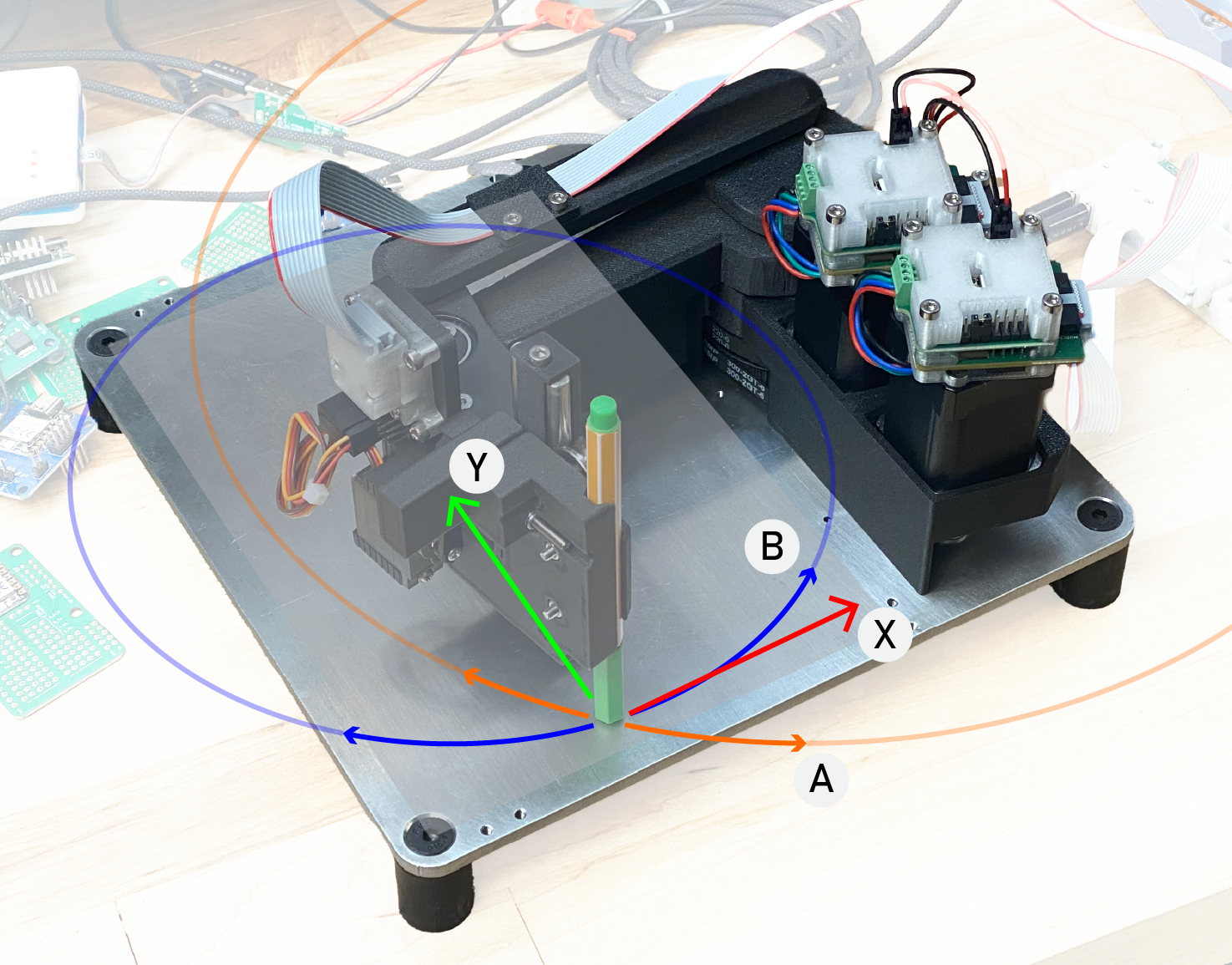
little guy machine, and its nonlinear kinematics where motion of the tool-tip in cartesian space is composed of arcs traversed by the machine’s two arms, which are connected to one another with rotary joints.
little guy drawing a test .svg — a small kinematics bug is present in the lower right corner of the drawing; defining transforms in Python can make debugging these errors simpler.
2.5.4.8 Bed Level Corrector
In FFF 3D printing it is critical that print beds are well aligned with the machine’s motion system so that the first layer of a print is of uniform thickness. However, beds often warp or are slightly misaligned with the cartesian side of the machine.
To correct for this, it is common to apply a transform to the system that adds offset in the z-axis which depends on the systems’ position in xy. I developed the Bed Leveling MAXL block for this, which applies a planar function (whose parameters have been fit to measurements) to a stream of z-points, based on measurements in the stream of x and y points.
The bed level corrector is used in-line with z-axis motion, and also reads xy states, using those to interpolate through a bed correction map and add the offset correction to the stream of z points. See Section 2.7.3 for a detailed look at how the leveller is operated and integrated.
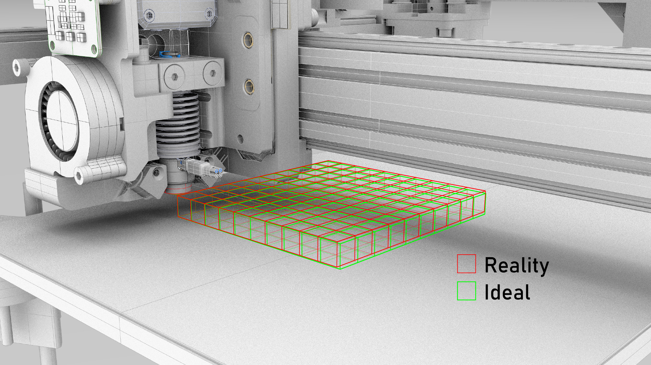
2.5.4.9 Spline Interpolator
Normally the terminal end of a MAXL system, the spline interpolator follows the logic outlined in Section 2.5.3 to generate interpolated \(p(t), v(t), a(t)\) and \(j(t)\) values. In this thesis, these are used by the motor controller in Section 4.4 as position and velocity control inputs.
Notably the interpolated spline outputs are not connected to lower layer hardware drivers hardware using Pipes, instead they are integrated directly within firmwares. This represents a performance limit in the system: interpolated outputs often need to be sampled at upwards of \(15 \text{kHz}\), which is too fast for OSAP’s internal runtime to process even between two ports in the same runtime.
2.6 Comparisons to Other Systems Integration Architectures
Now that we have covered background in networks, machine architectures, and also explained how OSAP, PIPES and MAXL all work together, I would like to draw a few clear differences between these architectures and those that are available in the state-of-the-art. First this will focus on the set of distributed architectures themselves, and then on their relation to machine interfaces and applications more directly.
2.6.1 Other Distributed Systems and PIPES / OSAP
PIPES and OSAP combine idea from many of these pieces of work but eschew a lot of the internal steps. These are design choices and are opinionated towards the particular set of constraints that I found while carrying out the other work in this thesis. While I make a clear architectural comparison between my systems and those surveyed above here, evaluating them rigorously against other distributed systems architectures more broadly is not the point of this thesis. Instead I show in Section 2.7 how they are uniquely suited to the challenge of “replacing” GCode with a software-defined alternative, and then extending into applications for model-based control. In 2.8, I relay what this particular set of trade-offs can teach us about systems integration tooling in a broader context. In particular, 2.8.5 discusses how the unique architectural arrangements of OSAP, PIPES and MAXL stack up such that distributed systems can be designed against their network constraints.
2.6.1.1 Function-Defined Interfaces, Typing, and Discovery
PIPES is code-first; device APIs define data schemas and these are sourced from devices into proxies so that systems can be designed using those APIS. Most middlewares are schema-first; systems-level data schemas are designed in Interface Description Languages (IDLs) and then device programs are built to interact with those.
OMG-DDS, ZeroMW and most of the serialization tools from Section 2.2.3.3 (ProtoBuf, Capn’ Proto) rely on centralized definitions of structs that are compiled at a systems level into a common set of serialized representations “on-the-wire.” This is known as schema-first or middle-out systems design: interfaces are designed ahead of time at the middleware layer and then software modules are written to adhere to those schema. The approach works well when systems authors have complete control over the contents of their systems or have complete documentation of the schema used by imported devices, but it can lead to misconfigurations if documentation are not available, are not followed properly or if parts of the system are updated without reflecting those changes in other components. These schemes also have limited discovery.
PIPES is of the code-first opinion. It relies on a unified set of core data types, but uses the host languages’ own typing system to define the schema that is required for each function (see Section 2.4.2 and 2.4.3). So, rather than specifying exactly how each device should interact with the system (either designing or trying to anticipate system requirements first and then configuring device software to suit) module authors can write generic functional APIs in the same style as they would were they to expose their module as a part of a software library. Those are then automatically wrapped into network-capable interfaces via the tools that I describe in Section 2.4.2. This is more akin to how modules in open source software commons like NPM and PIP34 are exposed to other programmers: designing good APIs is a well understood practice [123], [124] whereas designing network interfaces is less common. This is a relevant note with regards to later discussion on open source ecosystems (in Section 8.3, and alluded to in 1.4.1).
These types of tools are not completely novel; they are known as metaprogramming utilities and Capn’ Proto [125] includes one, others include Cista++ [126] and Serde in the Rust language [127]. The normal issue with these approaches is that the schemas are still required for interoperation: once we have our modules connected to the system, other participants still need to know how they should interact with them. PIPES uses proxies to solve this problem (in 2.4.4.2). Instead of generating schemas from remote data structures and then programming against those schemas, we write an intermediate schema (the function signature) and write interface functions — proxies — that serve as stand-ins for their remote counterparts. Those are typed against the user language’s native typing system. They can be called directly (generating remote procedure calls) when we are scripting, or used as handles to instruct PIPES’ manage to make connections between two functions (2.4.4.3).
The real underlying difference here is that PIPES devices and runtimes do not start up with any assumption about how they will interact with the larger system, their network configuration is initially stateless. Rather than configuring their internals against a data-based representation of the global system (an IDL), they each contain a small IDL that describes their local capabilities. Those are collected and then wired together at runtime to produce systems configurations, which I will elaborate on in Section 2.6.1.4.
2.6.1.2 Not Middleware, Underware
OSAP and PIPES align operating systems, networks, and program configurations and integrate more directly with embedded devices than state-of-the-art distributed systems. They do so by combining runtime-level ideas from very low-level systems like SpaceWire with system-scale ideas from very large systems (datacenters).
In each of the systems I surveyed in the background section on distributed programming models 2.2.3, software components are exposed to distributed systems via middlewares. Those run within software components and rely on existing operating systems to interface with other parts of the distributed program via OS-level networking drivers. This means that each is limited to network technologies that are suited to operating systems and they struggle to “cross the gap” between OS-level and embedded computing. For example MQTT relies on TCP/IP exclusively and ZeroMQ relies on Unix Sockets. DDS is more flexible, it technically runs on the “Real-Time Publish-Subscribe” protocol (RTPS, also from OMG) but RTPS is itself based on UDP/IP (and ROS runs on DDS…).
Those are relatively heavy protocols compared to the ones that are more commonly available in embedded devices that actually connect directly to hardware; larger microcontrollers can include IP-capable networking hardware but those are less common and more expensive than simpler link layers like UART, SPI or CAN bus. Middlewares also have lots of internal complexity for brokering and managing messages, buffers, topics, and Quality of Service (QoS); they themselves require tens of megabytes of RAM and relatively high speed processors to operate. This introduces a tension between realtime determinism and high performance computing; fast middlewares need both. For example ROS nodes that control servos directly rely on realtime-patched operating systems to maintain determinacy even though simpler microcontrollers are capable of the same core computing task were it not for the middleware’s own overhead [71]. These are often deployed on smaller Single Board Computers (SBCs) that fall in the category of “threshold computers,” they are not as powerful as typical OS-level devices but do run an OS, and they are not as deterministic as purely embedded codes but are much more deterministic than off-the-shelf operating systems.
To cross the gap into hardware, data from embedded devices are delivered over custom bridges like XRCE-DDS (eXtremely Resource Constrained Environments [65]), this bridge for OPC-UA on Arduino [68], or these RTOS (Realtime Operating Systems) for ROS [66] [67]: these do not run middlewares themselves, they instead provide tools to help build embedded bridges into middlewares. This is similar to the device virtualization strategies used by LabView from Section 2.2.3.4 and to FabNet, Klipper and MsgFlo from Section 2.2.4, whereas StepDance (2.2.4.6) is more genuinely distributed across embedded devices. Figure 2.24 below is adapted from [68] Figure 1, [65] Figure 1, and [67] Figure 4 - I add a colour code that approximately correlates to layers in the OSI model.
This is also related to how networks are integrated with circuits at a lower level; fieldbusses and IP-based network stacks are often connected to embedded devices using separate Network Integrated Controllers (NICS), which are subsequently connected to the device over a transparent data link through one of the microcontroller’s low-level communication peripherals. This can add some additional delay because data must make its way across this hidden link on trips into and out of the embedded device’s memory. In the systems that I developed, I chose primarily to use software defined network controllers - this is slightly lower level than the current scope, but it is discussed alongside the circuits that I developed in Section 3.4.
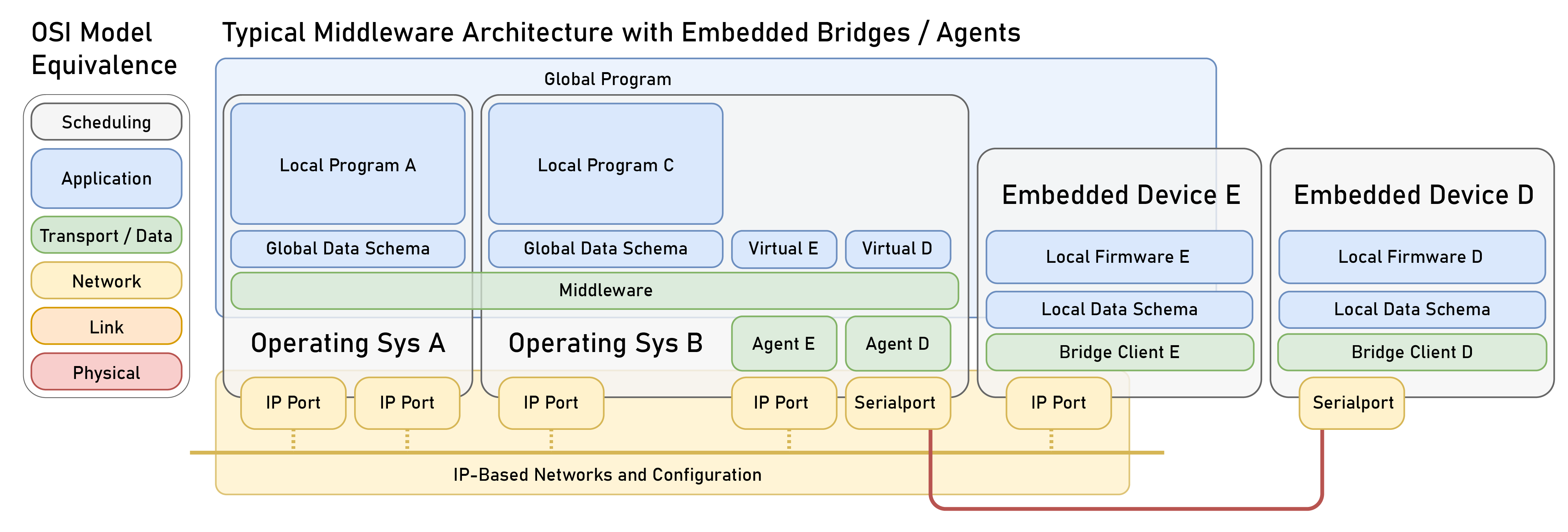
In OSAP and PIPES, software and networking links at both OS- and embedded-levels run within OSAP’s runtime (2.3.1, a version of which was written for cpp and Python); at the core of each runtime is a list of ports (which connect “up” into software) and a list of link gateways (which connect “out” into network segments). Each of those has an equivalent software interface that has tasks to run: OSAP schedules operation of links directly and can add and remove them and packets delivered to Pipes Functions can drive their operation via network interaction, Pipes Functions can also be remotely scheduled to run at fixed intervals or run by device programs directly. I compare this architecture to common middleware patterns in Figure 2.25.
That functionally replaces the OS with our own network-based runtime, so the analogy is that the systems in this chapter constitute underware rather than middleware. This is a strange arrangement because in embedded systems OSAP does constitute something like an RTOS35 but for Python codes OSAP runs on top of the pre-existing OS and then within the Python asyncio loop. However, it serves the purpose of causing software execution in both contexts to behave under the same scheduling rules and allows us to add more flexible, software-defined link layers to the network. It is difficult to write custom network drivers for an operating system but relatively easy to write simpler link layer drivers in embedded systems. OSAP’s runtime can use existing software APIs for network drivers to expose those links by wrapping them in Link Gateways, this includes IP-based network segments. However, this step requires software configuration of those links, see Section 2.3.1.2 for more discussion on how they are managed. OSAP’s internal network is also simpler than IP-based networks; it uses source routing (discussed in Section 2.2.2.2) to minimize computing overhead but still provides core services like naming and discovery (2.3.2.1), flow control (2.3.1) and time synchronization (2.3.2.2). I discuss its relation to other source-routed networks in Section 2.6.1.3.
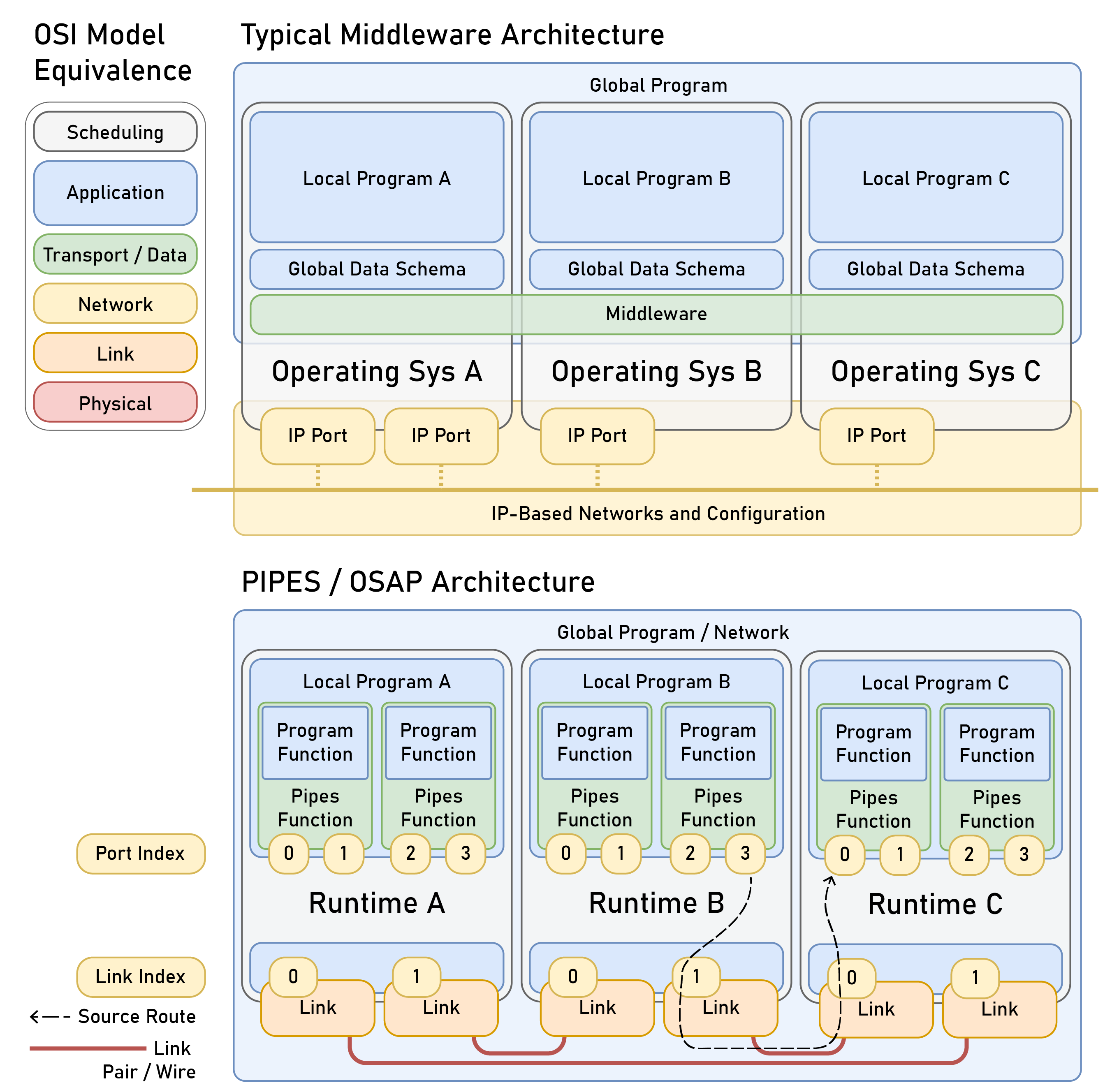
The distributed systems architectural model in the figure (2.25) above is adapted from [59] Figure 1.1. This figure helps to show how middleware-based systems act more like a shared memory layer than as a network configuration layer. The real value of different systems integration strategies can often come down to matters of opinion. The shared data model in many ways makes it easier to design systems overall because design of the interface (with an IDL) can be done ahead of time and then individual components can be designed around that layer. In many cases large computer programs are designed around their internal data representations, especially when many developers must build varying tools that each operate on e.g. the same database. So, IDL-based system representations also act more like normal computing systems where operation is fundamentally based on reading and writing data structures in memory. In that sense middlewares follow the software designer’s normal ethos, which is to hide lower-level operation in abstracted layers [128]. But this approach also hides network operation: new code is added to the IDL to define quality of service, actual inter-device connections, etc. IP-based networks further obfuscate important networking details because the route that any given packet actually takes through the system is not explicitly configures. Key aspects of systems performance rely on understanding those configurations at a global level.
I will expand on how this compares to the PIPES / OSAP data model and configuration in Section 2.6.1.4; network paths for program data are configured explicitly. But first a look at source routing and SpaceWire, which is tightly related.
2.6.1.3 Source Routing and SpaceWire
OSAP is similar to SpaceWire at a network level, with a few key differences around link heterogeneity and how routers are operated on a packet level. SpaceWire also lacks global discovery and configuration.
The standout difference between middleware-based architectures and PIPES / OSAP is the use of source routing. I covered this type of network already in Section 2.2.2.2, the recap is that where packets in IP-based networks are routed based on their addresses (leaving it up to the routers to decide how the network should operate), packets in source-routed networks contain routing instructions: each has a map of instructions and so routers need only to follow these simple instructions in order to deliver the packets. Section 2.3.1.3 describes how this is implemented in OSAP.
In their core networking schemes OSAP is most similar to SpaceWire [42], [117], which uses source routing for very simple and robust networking on orbit and even further away, i.e. in the James Webb Space Telescope [129]. SpaceWire was derived from the IEEE 1355 specification for point-to-point serial interconnects for scalable parallel-processor interconnects and embedded networks [130], that was itself based on the Transputer, a microprocessor designed from scratch for parallel computing: each chip had a CPU, memory, and four serial connection links such that they could be wired together to form scalable compute meshes [131]. Today SpaceWire is being extended over fibre links to increase throughput for modern systems with SpaceFibre [132], which also adds more complete QoS configurations and improved time synchronization. Time sync in SpaceWire / SpaceFibre is based on broadcast synchronization pulses, a lower-level mechanism than OSAP’s distributed diffusion (from Section 2.3.2.2).
Both use point-to-point links and simple routing instructions, in SpaceWire instructions are a single-byte in length (one byte per port forwarding step) whereas OSAP uses two bytes, which extends the number of port indices available at each step and also uses a few bits to delineate different types of forwarding instructions. The actual routing operating in SpaceWire is also much lower level: they use a technique called wormhole routing where programmable gates in the router are physically switched based on network instructions and packets are passed directly through those wires [133]. This is faster and lower latency than OSAP, where links must capture entire packets and then ensure their data integrity before handing them to the runtime where they can be forwarded (this is known as store-and-forward routing). Notably, modern Ethernet switches implement cut-through switching which also allows the switch to begin forwarding a packet before the last byte of that packet has arrived [134].
SpaceWire / SpaceFibre do accommodate some mixed links, i.e. serialport-type links of varying speeds, Low Voltage Differential Signalling (LVDS) links, and optical fibres, but it is not as flexible as OSAP’s software defined link integration; from a use-case perspective it is clear why there are differences here.
Interestingly, SpaceWire also includes provision for destination-based addressing and routers also include tables for this, but they are quite small. Those tables can be configured with a Remote Memory Access Protocol (RMAP, [135], [136]) that is also proposed to be useful for other remote configurations i.e. of instrumentation on the network.
Mostly, configuration of SpaceWire networks is done with manually authored source routes that are configured ahead of time and compiled into device firmwares. This is easy to do when you are building a satellite very carefully over many years in well coordinated engineering teams but not very useful for ad hoc systems development; SpaceWire does not include any remote discovery services — those are too complex to load into the resource-constrained and radiation hardened devices where it is most often deployed (i.e. on FPGAs). OSAP and PIPES include these provisions for global systems configuration, as we will discuss next.
2.6.1.4 Global Configuration for Distributed Dataflow
PIPES trades operational complexity (which is less than that of other systems) for configuration complexity (which is greater). However, this enables global systems capture and configuration by overlapping programming models with network models.
In a few places above I mentioned the trade-off that source routing networks make: while they make operation of the network much simpler, configuration of the network becomes more complex. For example to define a data path between two components in PIPES / OSAP, we need to know the whole system graph: how devices are connected over the network and which ports each of our functions lie on. If we were to author these systems without a network and program discovery utilities, we would have to carefully trace both configurations from their source codes and physical network topologies and write those down in device firmwares. This is why I built OSAP’s discovery service (Section 2.3.2.1) and PIPES’ Systems Object Model (Section 2.4.4.1) and discovery routine for the same. They allow us to write connections in PIPES that map across data schemas and network addresses to write Pipes, the virtual wires that articulate how data flows through the system: these connect through program models and network models. Figure 2.4 from Section 2.3.1.3 shows the data structures of two of these Pipes, and explains how they are routed through the network. Section 2.4.4.3 describes how they are configured.
The trade is to add relatively compute-heavy high-level configuration patterns like the Model-View Controller (MVC, [89]; discussed in Section 2.2.3.5) and function discovery services (2.4.2) to very simple low-level operation patterns like source-routing and earliest-deadline scheduling (from [29], discussed in Section 2.2.2.1). These parts of PIPES and OSAP are actually much more complex and consume more program memory, RAM, and compute cycles (when they are running) than actual program operation. But configuration steps don’t happen very often, normally only once when the machine is first configured, or when it is edited.
It also changes the programming model; middleware-based distributed systems route program data according to topic labels, as I mentioned this is akin to building a shared data layer across components. PIPES systems do not explicitly have a shared data model; each device and function defines their own (except for a shared global set of serializations for atomic data types, see Section 2.4.3). To collect and use those schemas, I use functional proxies (Section 2.4.4.2) that are interacted with in high level configuration scripts: remote functions can be called directly using RPC semantics or configured as dataflow components and the entire system, including data routes and network topologies is represented to the programmer in the Systems Object Model. So, where middlewares abstract the actual data paths from applications, in PIPES they are explicitly configured.
This also relates to configurations for Quality of Service. In middlewares, QoS is defined per topic in the shared data model and managed by the middleware. In OSAP, the network layer is used only for transmitting messages under the earliest deadline scheduling technique and QoS is defined via PIPES at the application layer on a per-pipe basis, and can be configured remotely. Individual connections between functions are configured with time-to-live based priorities and transport types to specify whether connections should enforce delivery guarantees or not. This is a much simpler set of QoS configurations than exist in e.g. DDS but could be expanded in the future.
2.6.1.5 Comparisons to Other Hardware Dataflow Systems
While other hardware dataflow systems surveyed present visual programming interfaces and PIPES is purely code-based, they each require that flows between embedded devices pass through a central broker whereas PIPES is genuinely distributed.
I should relate this quickly to actual dataflow programming environments that I surveyed in Section 2.2.3.4, i.e. LabView, Node-RED and MsgFlo.
LabView and Node-RED run in central interpreters: dataflows are coordinated between software blocks in those interpreters and specialized blocks are described to gather or transmit messages to hardware over bridges in the same manner as the middlewares connect to hardware. PIPES uses distributed dataflow - rather than passing messages along a bridge into a virtual device, they can broadcast messages directly into the underyling network and direct them to any data sink in the system. This means that it is possible to configure a pipe between two embedded devices without any oversight from a central runtime, which is a potentially powerful tool for low-level systems configuration.
Another point is that those systems’ dataflow configurations cannot be read or modified remotely, meaning that composing a dataflow graph that spans multiple runtimes is not possible or must be done by hand. Nor do their runtimes themselves configure network links to other runtimes, they are standalone. The systems in this chapter work together to produce a global systems model (Section 2.4.4.1) that combines network configurations from OSAP with program configurations from PIPES, both of which are discovered automatically.
MsgFlo is more similar to OSAP and PIPES: it is more genuinely distributed and devices and their functions can be discovered, but there are still a few important differences. The first is that networking in MsgFlo is fundamentally based on MQTT and IoT and overall network performance is bottlenecked by MQTT brokers which can be quite slow; multiple milliseconds of latency or more depending on traffic and link conditions making it unsuitable for realtime tasks [69]. Even flows that are sent from within one device back to itself must travel up and then back down from MQTT brokers, whereas each PIPES device runs an OSAP runtime where data passed between two functions within the device is transmitted via pointer ownership (i.e faster even than memory transfer, although data still needs to be serialized and deserialized see 2.3.1). Another performance limit for MsgFlo is in serialization, which is based on JSON. Finally, device capabilities are manually configured with an endpoint descriptor class and messages are not strictly typed, so misconfigurations are possible, whereas PIPES wraps functions automatically and types their inputs and outputs.
Of course the real difference is that these systems actually render dataflow graphs such that they can be interacted with visually, which PIPES does not do. Instead configurations are written as Python scripts. I discuss building a UI for PIPES in the future in 2.9.3.2.
2.6.2 Systems Integration from Related Model-Based Control Research
Moving towards the actual task at hand, it is relevant to relate how the state-of-the-art in distributed systems architecture overlays on the state-of-the-art in model-based machine control. There are two excellent sources in this regard, they are discussed also in the motion control chapter’s background section 4.2.8. In that section I also point out that the researchers in both of these cases chose not to modify their machine’s existing controllers; the software that they built works on top of those controllers via their “feed override” settings, which are high-level handles that set velocity targets rather than updating motor control loops directly.
This represents a limit of closed or difficult to modify systems. In the first case, a commercial machine controller is extended in a multistep bridge that crosses a fieldbus, a digital-to-analog converter (DAC) and coaxial cable, back through an analog-to-digital converter (ADC) that is then bridged into LabVIEW where the author’s controller runs. They must also develop a method to predict the existing machine controller’s own internal dynamics because they are hidden otherwise, again recall the note on the hidden optimization (1.3.3). In the second example, the authors are even using their own custom control architecture but still rely on an embedded bridge and still split state and control representations across that bridge. In Section 4.2.9 I explain how the architectures in this chapter allow me to integrate model-based control more intimately with low level machine controllers. I show the benefits that this entails in Section 4.7 and also in 5.10 where those controllers are extended for 3D printing.
First is Ward’s work on CNC machining with model-based control from 2021 [137]. They use a commercial machining center and NC interpolator (the machine’s own controller) that is connected to a LabVIEW instance that is running their model-based controller. The interpolator is configured to expose some internal states (commanded and actual motor drive positions and velocities, spindle RPM and spindle current) and accept feed override commands via its internal ProfiBUS network. These are connected to four fast analog input / output modules that convert the ProfiBUS values to voltages (and vise-versa), which are subsequently connected via coaxial cables to a multi-channel digital acquisition device from National Instruments that is subsequently connected to the author’s controller in LabVIEW, which was discussed above. Ward reports that readings are taken at \(250\text{Hz}\) (the same rate as the interpolator’s own position control loop) and feed overrides are updated at \(100\text{Hz}\).
Then we have Xin Tong’s work on a similar system from 2025 [138], this runs in an architecture that is developed by the authors in an earlier paper (2020, [139]). The layout is similar but avoids the analog input/output step; the machine’s interpolator is connected to its drive motors via EtherCAT and this is subsequently connected to Beckhoff’s ADS (Automation Device Specification) system, a PC-based automation platform that bridges to EtherCAT over IP [140]. Feed rate override commands are sent back over the same bridge into the interpolator, and the system input-output loop runs at \(100\text{Hz}\) overall. I compare these systems performance to those that I develop in Section 2.7.9.
2.6.3 Comparisons to Other Machine Control Architectures
MAXL / PIPES is one step in a lineage of modular motion control frameworks, but is the first to use software-reconfigurable dataflow to describe motion controllers, the first to automatically reconcile firmware and network configurations against software specifications, and is unique in the way that it combines dataflow and scripting. Overall the framework is uniquely suited to enable the rapid development and deployment of model-based controllers across machines and processes.
OK, that was an extensive look through architectural differences in networks, distributed systems and programming models. Here I want to compare the actual motion control architecture that I develop in MAXL / PIPES to other machine-specific control architectures. The next chapter will begin with a summary of overall architectural deltas and an explanation of how they relate to the results from this chapter (Section 2.7.1).
In terms of control partitioning, this work is most similar to OOH and Klipper: most machine control and configuration is located in a Python script and remote devices follow simpler instructions. In MAXL / PIPES, motion control graphs are mostly configured in Python and then broadcast basis splines to motors while consuming data from remote sensors. The big difference is that machine configurations are made using graphs of dataflow blocks, time synchronization is done explicitly in the network layer, and I use basis splines rather than lower-level representations for motion. StepDance is also configured using dataflow blocks, but does so in firmware and doesn’t provide tools for remote capture of distributed systems.
Configuration of each of these systems is also nicely bundled in one easy-to-edit python program, but another key difference is that PIPES’ configurations are automatically compared to underlying hardware data schema to ascertain whether or not these configurations are valid or possible given the currently connected hardware. Additionally, those remote devices’ schemas are generated directly from source code and can be faithfully mirrored at the scripting level using automatically authored proxies, whereas none of the other machine architectures that I surveyed here include this functionality. That said it cannot detect actual hardware misconfigurations (like a mislabelled axis), but it still makes substantial improvements over i.e. ROS; as I discussed in Section 2.2.3.2 nearly one third of ROS bugs are data layer misconfigurations [73], [74].
The broader systems architecture in OSAP / PIPES simplifies some lower level configuration steps that are required in other machine systems; OOH and Klipper both require manual mapping between network addresses and controller configurations whereas OSAP’s network discovery step is combined with semantic naming schemes in PIPES to automatically find and match network configurations to software configurations: you can re-wire the machine’s network without re-defining the control program configuration.
MAXL / PIPES is also the first to combine dataflow with scripting for machine control, whereas other systems use one or the other. In my master’s thesis [113] I developed a distributed dataflow machine controller that was entirely based on dataflow, it was difficult to operate hardware using this system because every small operation had to be authored using dataflow blocks even though high level machine operation is often sequential (do this, then do that…). Being able to operate dataflow blocks — and their virtual representations as proxies — in scripting routines is extremely useful, as I will describe in Section 2.7. At the same time, being able to describe static dataflow configurations for realtime control is valuable because it allows us to change remote components of the system without orchestrating that operation from within an operating system. The clearest example of this is in data collection, where we configure remote functions to continuously transmit data at fixed time intervals (2.7.7).
This data collection capability is also missing from most other machine architectures, or where it is possible it is integrated directly within GCode interpreters themselves rather than being exposed as a more flexible configuration step. In Section 2.6.2 I covered two examples of state-of-the-art methods where machine controllers were extended to include realtime data collection, those both develop ad hoc systems that interoperate but do not directly integrate with machine controllers themselves whereas PIPES allows these configurations to appear in the same programming model where the controller itself is built. In Chapter 4 I show how MAXL / PIPES is extended to integrate these data more intimately with machine control, and then Chapter 5 and Chapter 6 extend those methods to cover process control for 3D printing and process inspection in CNC machining.
Finally, adding dataflow without hiding simpler RPC calls turns out to be invaluable for tasks like model building and low-level controller tuning (I provide examples of each in Section 2.7.4), and for building simpler machine controllers (examples in 2.7.10).
2.7 Deploying OSAP, PIPES and MAXL
2.7.1 Architectural Deltas and Results
I will start this section by summarizing the comparison in 2.6 between the OSAP / PIPES / MAXL stack of architectural contributions and similar state-of-the-art technologies and articulating how those deltas lead to the results in this section. As I mentioned near the end of this chapter’s introduction (2.1.3.1), the primary challenge with these systems lies in developing something that is descriptive enough to capture and flexibly configure complex distributed systems but simple enough to be deployed in our smallest components without substantially hindering their performance.
In Section 2.6.1.1 I explained that this work uses a code-first paradigm for interface development and how that differs from most state-of-the-art systems’ schema-first style. This difference helps us develop modules that can be deployed in multiple systems because it decouples device development from systems development. Most other distributed systems are defined first at the systems level with an Interface Design Language and devices are subsequently attached to that; if the IDL is modified the devices may need to be updated. Section 2.7.2 shows how I assemble systems from the device layer up and Sections 2.7.5 2.7.10 show how I use this property to re-use devices in multiple machines without modifying device-specific firmwares.
Rather than integrating on top of existing operating systems, OSAP builds a common runtime for high- and low-level devices. Instead of relying on OS-level network drivers it uses APIs to integrate software-defined links and then includes a simple networking protocol (in source routing) to build networks from links. This brings operation of the network back into the purview of the distributed system itself rather than riding on top of IP-based backbones as I described in Section 2.6.1.2. To keep operation of these networks lightweight, I borrow ideas from extremely simple and redundant systems e.g. those used in spacecraft as I related in Section 2.6.1.3.
This enables tighter integration of embedded devices within our systems; Figure 2.24 in 2.6.1.2 shows how bridges are used in the state-of-the-art to integrate embedded devices and Figure 2.25 in the same section shows how embedded runtimes are integrated directly into distributed PIPES / OSAP systems. In Section 2.6.2 I gave some clear examples of how this type of integration is managed in the state-of-the-art; in each of those cases, integration between low-level devices and “smarter” controllers was indirect. In Section 2.7.8 I explain how similar systems in the MAXL / PIPES / OSAP stack are assembled and represented in a single coherent architecture, and Section 2.7.9 analyzes timing performance throughout.
Much of this work is enabled also by time synchronization across levels and a careful separating of time scales between the operating system and embedded devices. Besides enabling us to deploy more powerful compute devices for core planning tasks, moving trajectory planner into the operating system helps to make them more transparent. Doing so was posed as a problem in earlier discussion of the hidden optimization 1.3.3; in Sections 2.7.6 and 2.7.7 I describe results that emerge from that capability.
The low-level networking scheme and code-first data schema would make for difficult system set up if we did not subsequently include systems for remote discovery and configuration: here we can borrow ideas from much larger distributed systems like datacenters e.g., the model-view controller, distributed clock synchronization and software-defined networking, those were covered in Section 2.2.3.5. These tools are used throughout systems in the thesis. With the additional step taken by MAXL to develop motion control using a composable set of dataflow blocks, we can re-use devices across machine projects (2.7.5), re-use software and control modules and rapidly reconfigure software defined controllers (2.7.4), and re-use core motion control modules across variable kinematics (in Section 2.7.5.1).
Overall this makes for tighter integration across the layers of machine control that GCode is used to separate; it lets us transition from GCodes to just… codes, on networks.
2.7.2 Bootstrapped Systems Assembly
So, a lot of this architectural work was organized around the goal of making the development of new machines more straightforward and flexible. In model-based machine building and in systems assembly more generally we often have the problem that assembly can’t happen all at once; we need to build piece-by-piece: components are modelled, configured, and then integrated into subassemblies, those integrate into other subassemblies and so on. Being able to do this “smoothly” is important; with e.g. GCode interpreters we cannot do systems integration tests using the GCode interface itself, we have to manage multiple code bases and systems “views” etc. Those interfaces also make it difficult to subsequently reconfigure hardware for spot tests, for example in the 3D printing work here the printer runs intermittently as a printer and as a materials testing machine. Both the printer and the milling machine are used to generate data for their own kinematic model fits, etc. In these cases and in other debugging situations it is valuable to be able to quickly develop new subroutines and systems that run only parts of the hardware.
Here I want to work through the example of my retrofit of the FrankenPrusa (Section 5.4.2), showing how I bootstrap controllers as systems of systems. This is relevant both for the modelling methods that will come in Chapter 4 and Chapter 5, but also to see the results of our new systems integration tools.
2.7.2.1 Capturing the Physical Layer
Firstly we need to outfit our hardware with the embedded devices that we will use to control them. I explain this process in more detail in Section 3.6.2, but I include Figure 2.26 here for a quick example. When I did the Prusa \(\rightarrow\) FrankenPrusa retrofit I was surprised to see how small the set of “terminal” electrical connections to the machine was (top left of Fig. 2.26). This small set of wires is the thin interface that the system senses and controls the machine through.
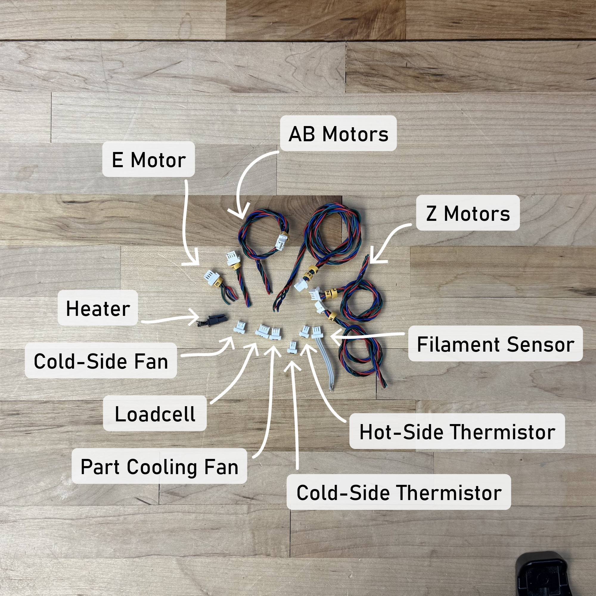
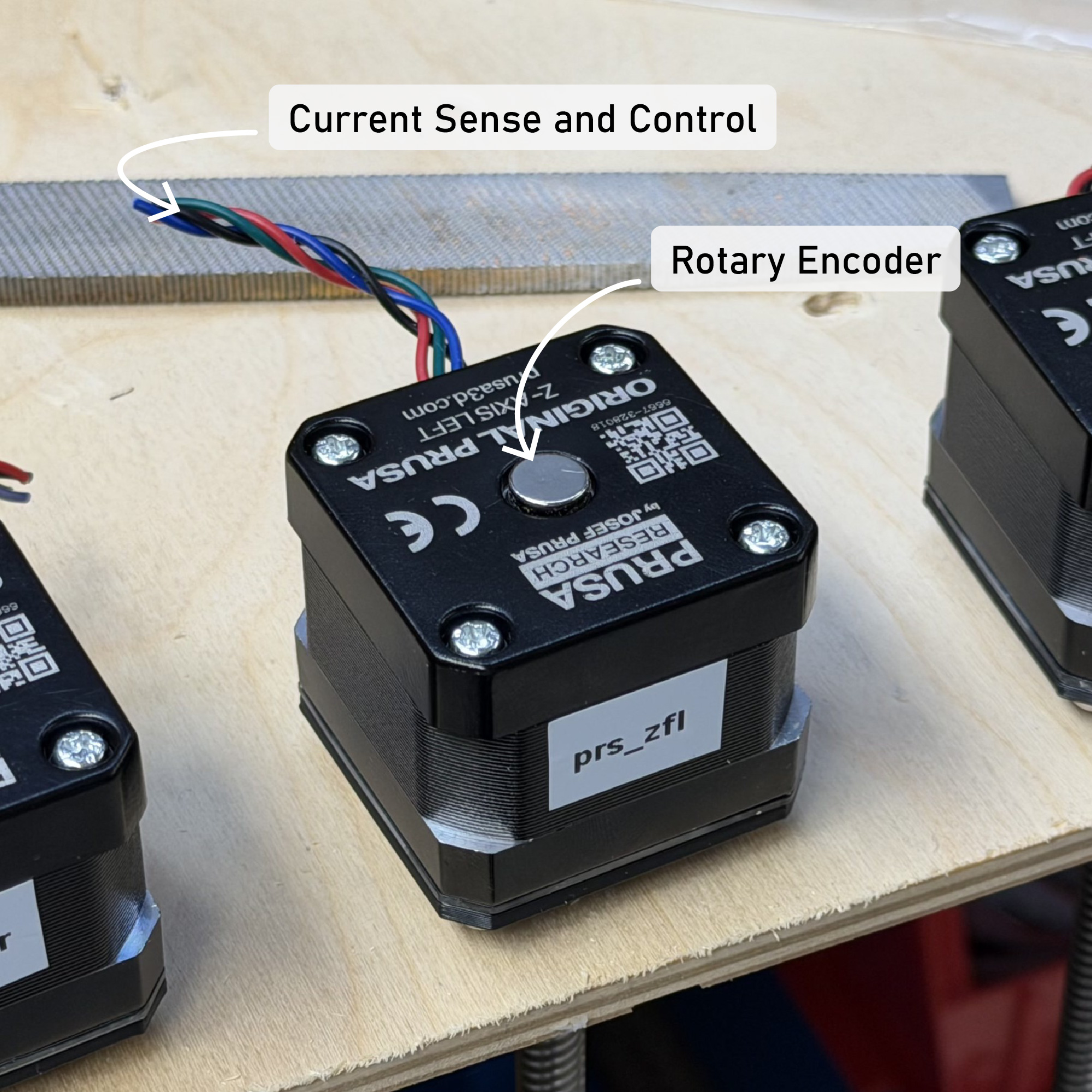
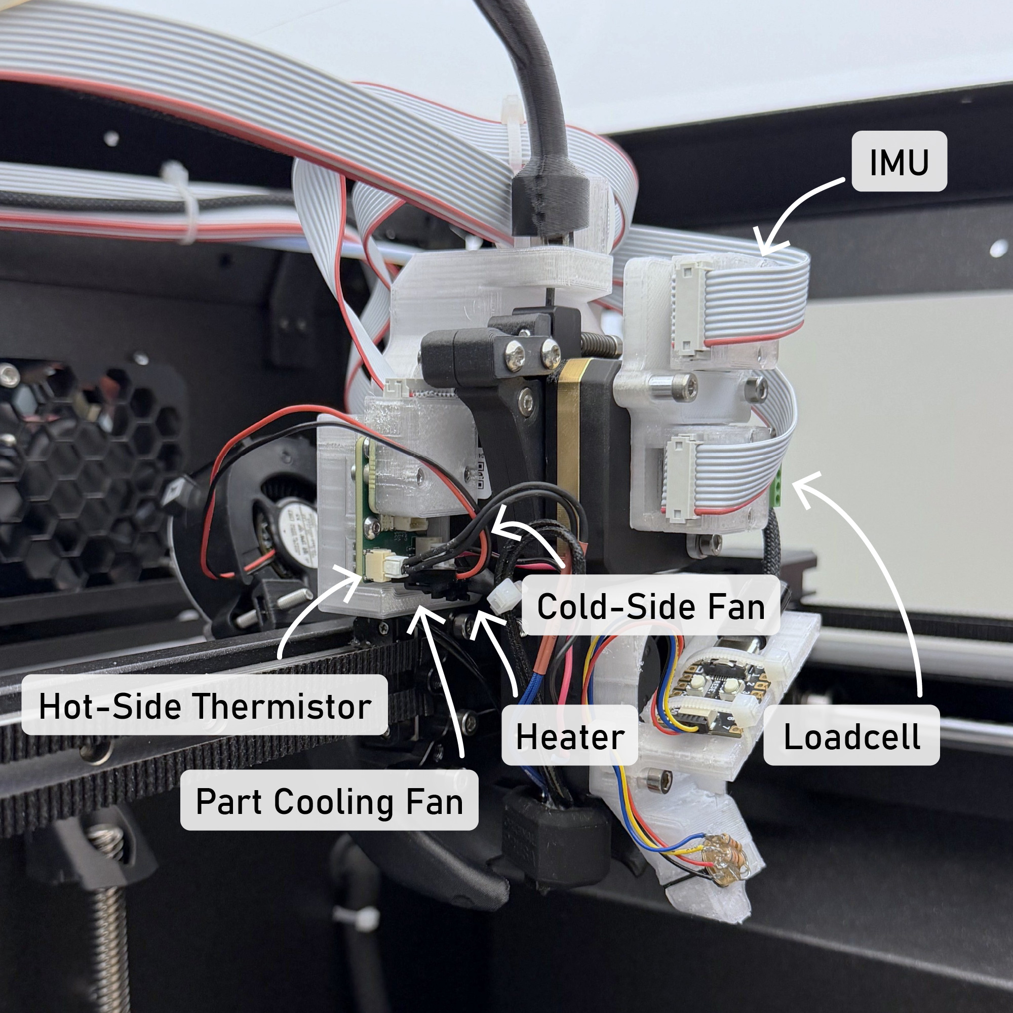
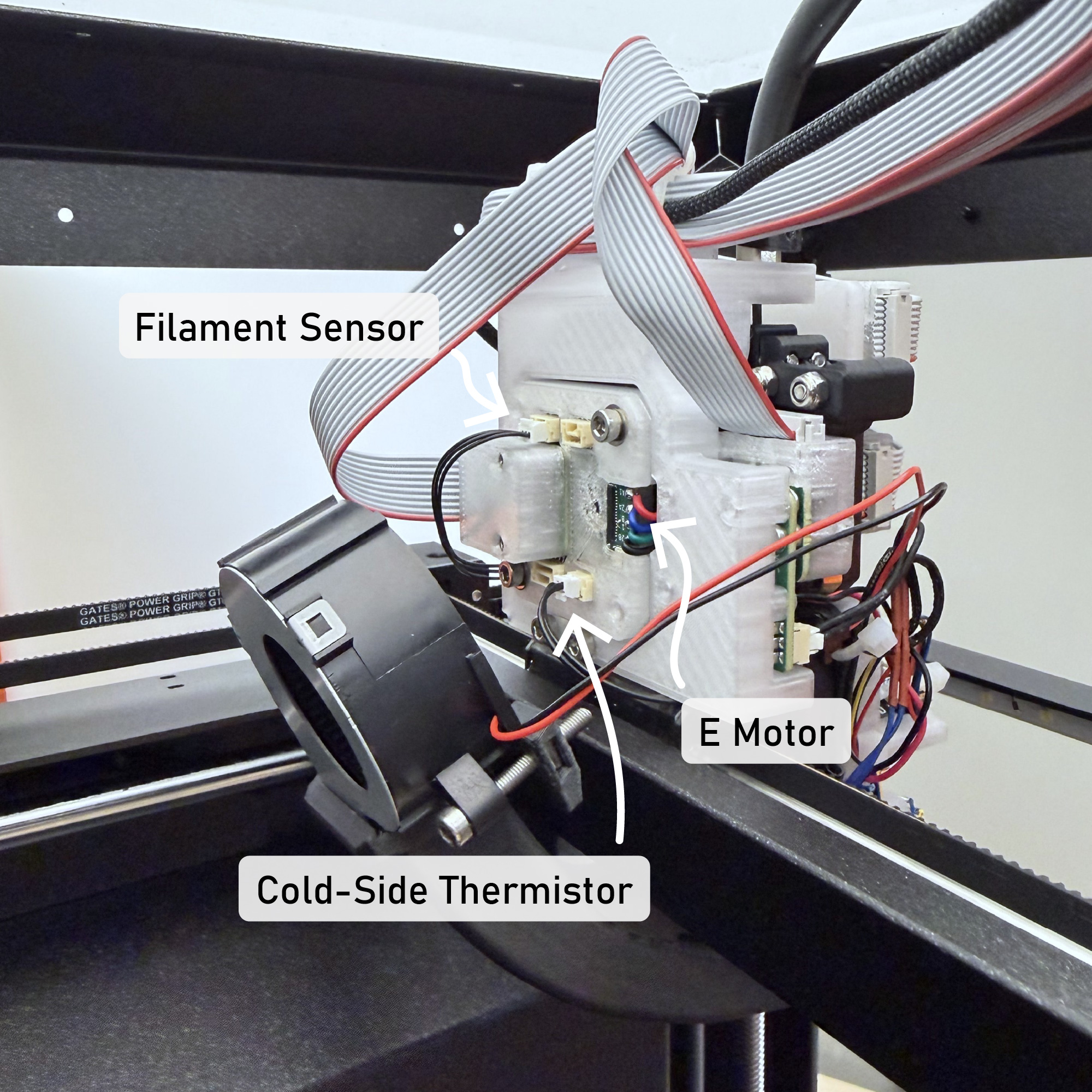
Here I also mount circuits adjacent to the hardware that they control. For the FrankenPrusa this required that I develop some new bracketry. Industrially it is more common to mount control boards in an electrical cabinet (on DIN rails) and build a wiring harness between the cabinet and hardware. The harness from the Prusa appears in Figure 3.21 later on, alongside more discussion on the topic; the short version is that as circuit modules become smaller they approximate the size of the connectors we use to interface to hardware anyway — especially for sensors. In any case this layer is not required by the computing architecture, it is just the way that I have elected to manage this step.
To each motor I also add a magnet to the back side of the shaft, this is how the motor controller reads rotor position (which is required for closed-loop control). Some more advanced motor controllers can sense rotor angle from electrical signals alone, but I won’t get into that here.
2.7.2.2 From Hardware to Software with Firmware
Once devices are mounted, we need to write the firmware that will run within each. At this layer we are effectively writing software interfaces that describe both what our hardware can do (by exposing APIs) and what they are, i.e. naming them.
I tried overall to maintain just one firmware for each circuit module and then use higher level configuration to assemble them into systems. For devices that have one clear purpose (the motor controller, load cell sensor, and accelerometer) I was successful in this regard. But there are two devices that I developed to be repurposed for multiple tasks where this was more challenging: the H-Bridge module and Deadbugger (see Section 3.2) are both “generic” hardware that I use for multiple tasks. For example the H-Bridge module can be used to drive DC motors, LEDs, or heaters (generic DC loads), but each of those hardware configurations requires slightly different firmware. In the FrankenPrusa I use it to control the nozzle heater, hotend fan, and part cooling fan and so here I load the version of its firmware that is set up for those tasks.
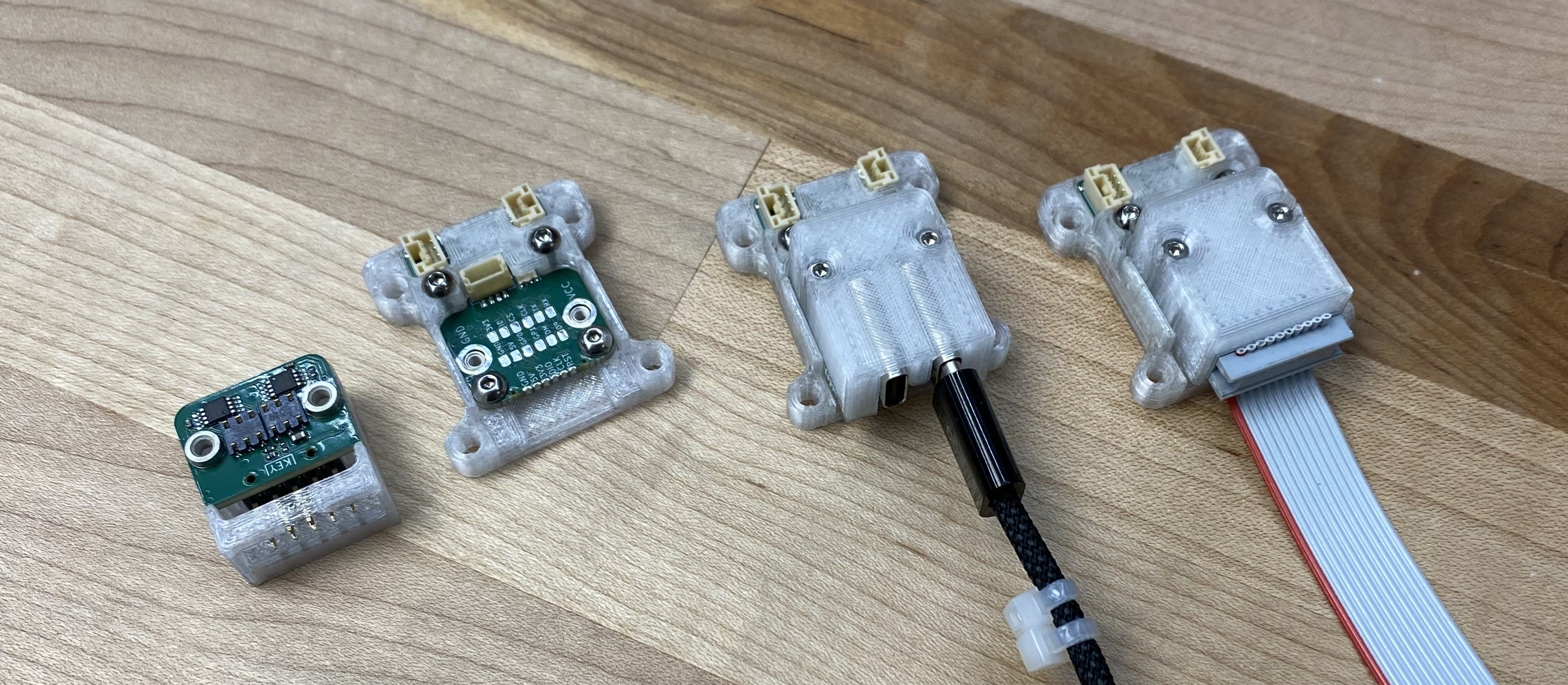
The second step here is in configuring each device’s OSAP runtime to attach the link gateways that will be used in the particular system, Listing 2.9 in Section 2.3.1.2 shows how this is done: different gateways can be instantiated according to a compile-time configuration. I will note that we do not need to give the device a network address — those are discovered — but we do need to set up the runtime such that it will load the relevant driver. This is required with the devices that I use because I also built the modules to be physically reconfigurable for different network types with “backpacks” (see Section 3.3 and Figure 2.27). Circuits that are statically configured with multiple network interfaces could simply add multiple gateways to the runtime.
Finally, each device should be named in a manner that is semantically meaningful at a systems level, for example the A and B motors in the FrankenPrusa are named prs_a and prs_b respectively. These will become software handles in the next step. In Section 2.3.1.1 I described how that is managed in the set up of the OSAP runtime: firmwares can define a static name via a compile-time configuration, but names can also be written remotely and are stored in non-volatile memory. So, it is possible to eschew this firmware configuration and do instead an initial set up step where networks are discovered, default device names are found, and then they are updated using a remote software interface.
2.7.2.3 Making Network Connections
So, by now we have hardware mounted and firmwares configured. Of course, we also connect networks; besides defining which link gateways will be instantiated in each device runtime there is no additional configuration other than physically connecting all the network links and mounting whichever intermediate routing devices or hubs (see Section 3.5) will be used. To be able to isolate certain subsystems later on, I normally organize network topologies according to sensible decompositions in this regard: for example the hub in Figure 3.12 connects to the top half of the RheoPrinter: the nozzle heater, load cell, A, B and extruder motors. When I run material flow tests, I only need to have this device connected to the Python workstation and script. In that figure I have labelled the physical ports according to which device is connected, but this is not a required step: again, network addresses are discovered and reconciled with the semantically meaningful names that I just described at runtime. Certainly it is still useful to label ports for other unforeseen debugging steps, e.g. in the case of physical port failure it is then easier to swap devices between ports to identify which end of the wire is broken.
To connect out of the operating system, we need also to tell the Python script where it should look for devices. This is a similar step to the firmware link gateway configuration. In the OS we can add some additional discovery tooling. For example Listing 2.6 shows a utility that I use to search for connected USB CDC devices that the OS has found, and automatically built new link gateways for each that matches a list of device IDs (a USB-layer identifier that identifies e.g. which type of microcontroller is connected per-port) that match to a list of known device IDs. This tooling (which is software-defined) prevents us from having to reconfigure the runtime every time (for example) the operating system re-assigns logical ports to hardware.
2.7.2.4 Collecting Device Schemas
OK, we have our devices connected to a Python runtime, but we need to know how to program against them. This is where we use the systems discovery routines and the PIPES SOM (Section 2.4.4.1) to automatically build that programming schema. To build those, I developed a generic Python script that wakes up, connects to any devices that are attached to the operating system, scans the network for remote devices, and then collects the SOM and writes proxies (Section 2.4.4.2) against it.
This results in one software interface for each type of remote runtime in the system. So for example all motors share the same proxy because their APIs are identical, and then systems can be collected by defining which device name should match to each software object. An example proxy (for the load cell) is in Listing 2.24, and Listing 2.29 shows how I typically assemble those into higher level systems that are described as software objects.
2.7.2.5 Per-Device Calibrations and Models
But developing complete hardware objects for systems is not a required step, it is just a useful abstraction that can be added to manage more complex projects. For example before we can author complete systems, we often need to make smaller subsystems and models. The motor provides two good examples; each requires that we run an encoder calibration routine (see Section 4.4.0.1) and then a motor modelling routine (see Section 4.5.1). For each of these I have standalone Python scripts that connect to one motor only and perform the relevant data collection / fitting routines.
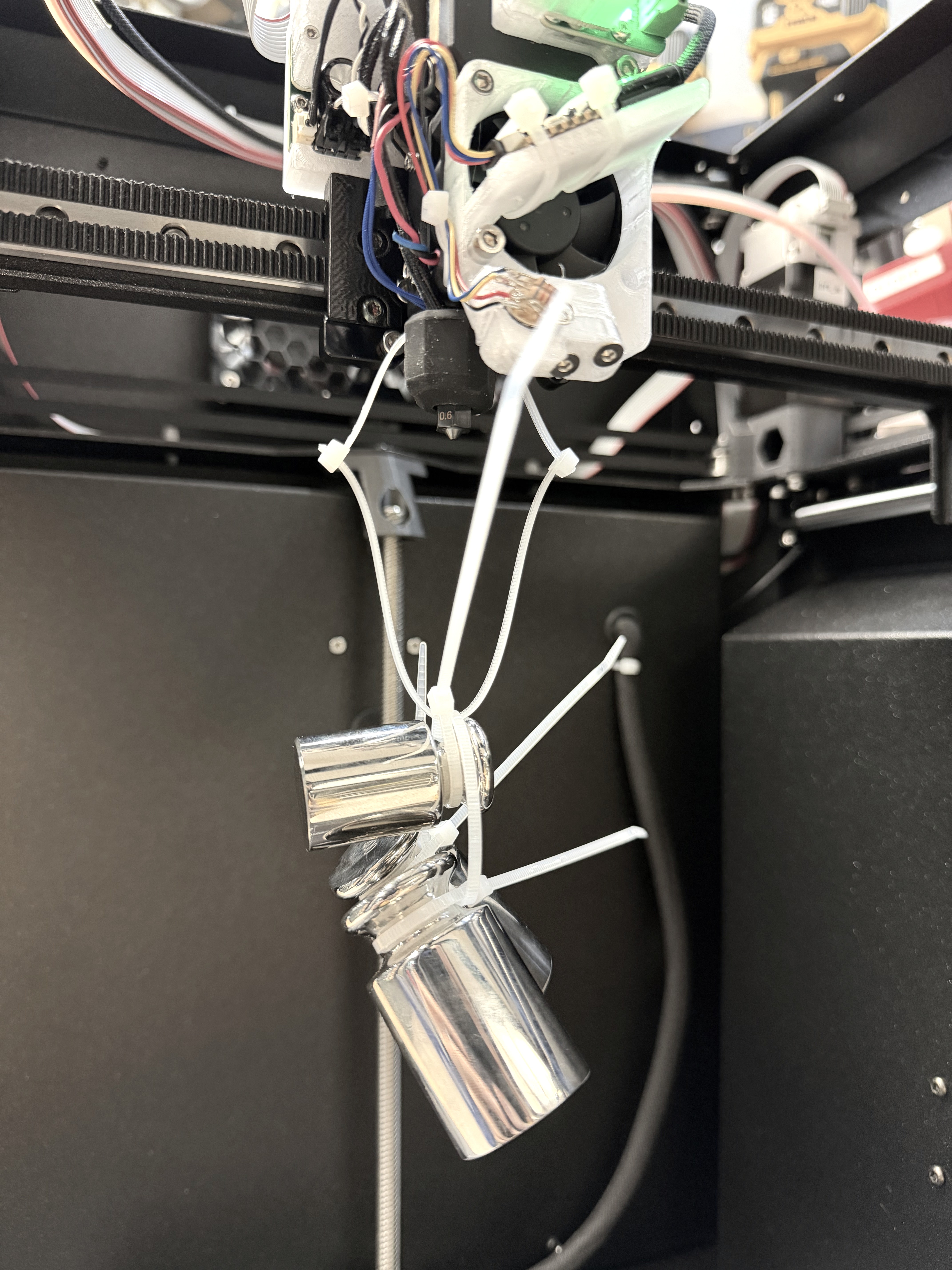
# in 'run_calibrator_loadcell.py`
# ...
loadcell_name = "prs_ldcl"
# ...
async def main():
    # ...
    osap, manager = await network_tools_setup()
    # ...
    # discover and instantiate the loadcell alone,
    await manager.refresh_system()
    loadcell = LoadcellCs5530D21(manager, loadcell_name)

    # set prior calibration if testing, or ignore if not,
    loadcell_slope = -0.000206289
    loadcell_offset = -12.6785
    await loadcell.set_calibration_params(loadcell_slope, loadcell_offset)

    # just poll and print values,
    while True:
        await asyncio.sleep(0.25)
        stamp, reading = await loadcell.get_raw_loadcell_reading()
        stamp, calibd = await loadcell.get_calibrated_reading()
        r0 = r0 * a0 + reading * (1.0 - a0)
        r1 = r1 * a1 + reading * (1.0 - a1)
        print(F"({calibd:6.3f}): \t{reading}, {r0:.0f} @ 0.95, {r1:.0f} @ 0.99")
Another good example is load cell calibration, which is a similar standalone script; an abbreviated definition of that is in Listing 2.28. This one is quite simple, I read data from the sensor, filter it slightly, and print it out to the terminal. I then attach weights to the load cell and make notes (with a pen!) for raw readings at each weight. Those go into another script that fits a linear and offset term for the load cell, which I write down in the printer’s configuration file. Not everything has to be complex.
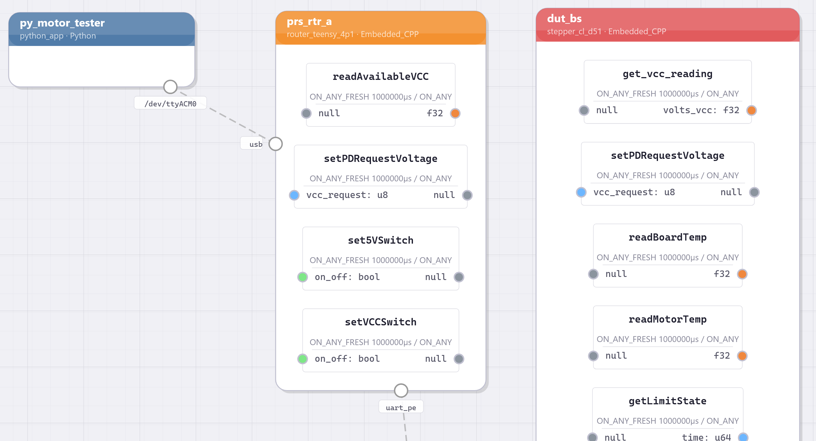
I have a litany of other such scripts, for example for tuning heater PIDs, testing networks and synchronization, debugging various devices, etc. In most machines, developing these routines is difficult because GCode does not contain standard codes to operate low-level hardware on a piecewise basis. Some other modular machine architectures do develop these interfaces, like Object Oriented Hardware and even the Duet Firmware (which provides an out-of-band interface, eschewing GCode itself for this step). But those require that software interfaces at a high level are developed to match embedded device APIs, which can lead to misconfigurations.
I invested a deal of time developing the underlying tools that enable the automatic collection and authorship of device proxies. That involved template programming in firmware to read function signatures against source code, automatically building network interfaces against those signatures, serialization routines for “almost any” data type, the network and PIPES discovery routines and graph traversal codes, etc. Those tools turned out to be invaluable, especially for firmware development because they automate the assembly of systems-wide software interfaces.
Although it is common to try to develop subcomponents in a principled way so that systems can be assembled bottom up, in reality we often need to edit low-level interfaces in response to emergent systems integration challenges. This was the case throughout my experience with the machines that I will show in this thesis; I developed firmwares alongside systems, for example realizing that I need to expose a lower level interface for a particular task, or a thinner one to reduce network loads. In the subsection on the closed-loop motor controller (4.4), I show two software interfaces: one is a rich set of debugging values that I used in motor modelling and MAXL debugging steps, and the other is a lighter set that I transmit from actuators while machines run for machine scale modelling. Instead of carefully writing network interfaces for each of these, I simply wrote new functions in firmware that returned different sets of values that were already present in the controller itself, and then updated proxies to match automatically.
2.7.2.6 Systems and Kinematic Configurations
Once piecewise devices are configured and calibrated (if required), we can start to build higher level systems descriptions. Listing 2.29 shows the Printer class that I use for the FrankenPrusa, it bundles devices in that machine into one logical object that can be used across flow tests, motion modelling tests, and to print parts themselves. Listing 2.30 shows how MAXL / PIPES connections can be established (and Pipes Classes / MAXL Blocks instantiated) within that class using the PIPES Manager’s functionality (as in Section 2.4.4.3) to define the machine’s kinematics.
2.7.2.7 Making and Maintaining Devices, Systems, Processes, and Workflows
Assembling systems-level software objects is roughly the terminal step of the bootstrapping process. At that point we have all the interfaces and calibrations required for subsequent work; in the next sections I will show in some more detail how each of these components are used to make machine models, operate machines, reconfigure them, etc.
Overall I hope that it is clear from this smaller set of examples how systems development cycles are improved with MAXL / PIPES and OSAP. I presented this in a bottom-up progression, but in reality development is nonlinear. The tools here are particularly useful in those cases; for example when device firmwares change, new proxies can be quickly written against them. When those are imported into scripts or systems that depend on them, changes to function signatures are reflected in the development environments that we use to author those systems. At the same time if firmwares are updated but proxies have not been changed to reflect that, misconfigurations are discovered during set up steps to alert the programmer that the underlying schema has changed.
In a broader industrial context, it is also unlikely that all of these components (firmwares, networks, systems) will be developed by one team or even one organization. In those cases I think that the clear separation of interfaces also shows clear value. Standalone proxies are probably most valuable to device developers and firmware authors to perform small unit tests or e.g. factory calibrations. It is a bonus that those same interfaces could be used by their customers during systems integration, where the same functions that are perhaps called via RPC during simple tests are then connected to realtime systems via PIPES dataflows. Because each is typed and described in the firmware itself, device manufacturers (or e.g. open source developers) may not even need to provide substantial documentation for their parts; if we can maintain standard protocols for self-describing hardware the world of mechatronic systems could become “plug-and-play,” as I will elaborate on in Section 8.3
# in 'machines/printer.py'
# ...
# this class is written automatically against the PIPES SOM
from proxies.printer.stepper_cl_d51 import StepperClD51
# ...
# this class is authored for the particular system,
class Printer:
    def __init__(self, osap: OSAP,
                 manager: MetaManager,
                 config: PrinterSetupConfig):
        # ...
        # in some cases the class will run partial hardware,
        self.mot_a: StepperClD51 | None = None
        self.mot_b: StepperClD51 | None = None
        # ...
        # instantiate local Pipes Classes / MAXL Blocks,
        self.dof_x = MAXLOneDOF(xy_dofs_max_vel, xy_dofs_max_acc, 1.0)
        self.dof_y = MAXLOneDOF(xy_dofs_max_vel, xy_dofs_max_acc, 1.0)
        self.corexy = MAXLCoreXY(xy_dofs_out_scalar)
        # ...
    # ...
    async def setup_devices(self):
        # ...
        # ensure network map is up-to-date,
        await self.manager.refresh_system()
        # ...
        # now we can get hardware,
        if self.config.use_xy:
            self.mot_a = StepperClD51(self.manager, self.config.motor_a_name)
            self.mot_b = StepperClD51(self.manager, self.config.motor_b_name)
        # ...
    # to check at runtime if devices are present,
    def require_ab_motors(self):
        assert self.mot_a is not None
        assert self.mot_b is not None
        return self.mot_a, self.mot_b
# ... continued ...# in 'machines/printer.py'
class Printer:
# ...
async def setup_kinematics(self):
# ...
# set up corexy block to wait for all new inputs from both gates
self.corexy.fwds_transform.set_input_mode('all_fresh')
# xy dofs -> corexy,
await self.manager.connect(
self.dof_x.on_new_pt, # output
self.corexy.fwds_transform, # input
"0, 1", "0, 1") # argument mapping
await self.manager.connect(
self.dof_y.on_new_pt,
self.corexy.fwds_transform,
"1", "2")
# ...
# now do hardware downlink,
if self.config.use_xy:
mot_a, mot_b = self.require_ab_motors()
await self.manager.connect(
self.corexy.fwds_transform,
mot_b._maxl_add_control_point_proxy,
"0, 1", "0, 1")
await self.manager.connect(
self.corexy.fwds_transform,
mot_a._maxl_add_control_point_proxy,
"0, 2", "0, 1")
# ... 2.7.3 From GCodes to Code
Having shown how machine systems are assembled with these new tools, I want to carry on by explaining how these patterns (some of which are new, some of which are essentially Peek and Moyer’s Object Oriented Hardware patterns [13] [12]) are used to operate and program machines. Here I will still be looking “inside” the system, i.e. at a task that is classically run within a GCode interpreter.
This is “Bed Levelling;” as I explained in Section 2.5.4.8, it is important that 3D printers’ motion systems are well aligned in-plane with their print beds, but beds are often slightly skewed or warped. To correct these errors we can apply a position-varying offset to the Z axis of the machine according to measurements made of the bed’s surface.
This is an excellent example of a capability that is normally difficult to add to machines because interpreters are difficult to extend, as I showed in Section 2.2.1. It involves precise timing between sensors and motion systems (to measure the bed surface), updates to some of the machine’s kinematics, and that we perform some more advanced mathematics (to fit a plane or other offset correcting function to data). It also requires that we develop a new function to perform the routine, so in a GCode interpreter we would have to author all these steps in firmware alongside the rest of the machine controller’s functions, mode-switch the machine to run the subroutine, store and fit data, etc — and somehow relay to machine users which Gxx string to add to their programs in order to trigger the new code.
@pipes_class_implementer
class MAXLBedLevel:
    def __init__(self, a: float, b: float):
        # params
        self.a = a
        self.b = b

    # xyz -> z + correction
    def on_new_pt(
            self, time: int,
            x: float, y: float, z: float) -> Tuple[int, float]:
        # apply planar correction, return (time, z)
        return time, x * self.a + y * self.b + z

    # update the fit,
    def apply_params(self, a: float, b: float):
        self.a = a
        self.b = b

    # calculate a, b params
    def _do_fit(self, pts):
        # reshape points,
        n = len(pts)
        a_mat = np.zeros((n, 3))
        b_mat = np.zeros((n, ))

        a_mat[:, 0] = pts[:, 0]
        a_mat[:, 1] = pts[:, 1]
        a_mat[:, 2] = 1

        b_mat[:] = pts[:, 2]

        # fit using numpy,
        a, b, c = np.linalg.pinv(a_mat) @ b_mat

        # return a, b and the offset,
        soln_pts = pts[:, 0] * a + pts[:, 1] * b + c
        soln_pts = np.column_stack((pts[:, 0], pts[:, 1], soln_pts))
        return a, b, c
Here we do this in a few contained steps. I show in Listing 2.31 how the leveler’s correction logic works: the block has a, b parameters for the correcting plane, and is connected into the MAXL pipeline through the on_new_pt function, which intercepts the machine’s x, y and z positions. It uses the x, y position to evaluate the plane function at that point and adds the offset to the existing z offset. Because these are encoded in time, any upstream or downstream acceleration control that is applied is outside our concern.
So, part of the block is in the MAXL stream, but it also has “normal” function interfaces that can be used to perform the fitting routine and apply updated parameters. To collect the points for the fit, we need to coordinate machine motion with sensing. Here, time-aligned data and MAXL’s blocks are useful again. In Figure 2.11 and Listing 2.20 I show the OneDOF block. The OneDOF block contains logic for homing an axis, as I described in Section 2.5.4.2. That essentially involves running the axis in a velocity control mode until a switch signal appears (via PIPES) to indicate that it has reached a known position (its “endstop”). Bottling this capability into the OneDOF was invaluable for machine development here because we often want to apply homing routines on either actuator axes or motion axes. For example the CoreXY system in the printer homes in X and then Y, but the actuators are in A, B. In this case the OneDOF block is located before the CoreXY block.
There are four of these in total to control the Z axis of the printer: one of them is located ahead of the bed levelling tool (after the motion planner), and the other three are in-between the levelling tool’s output and the individual motors because each of them occasionally needs to be controlled independently. When the bed initially homes to its starting position we need to ensure that they are synchronized in position with one another; all three are homed to their respective endstop simultaneously.
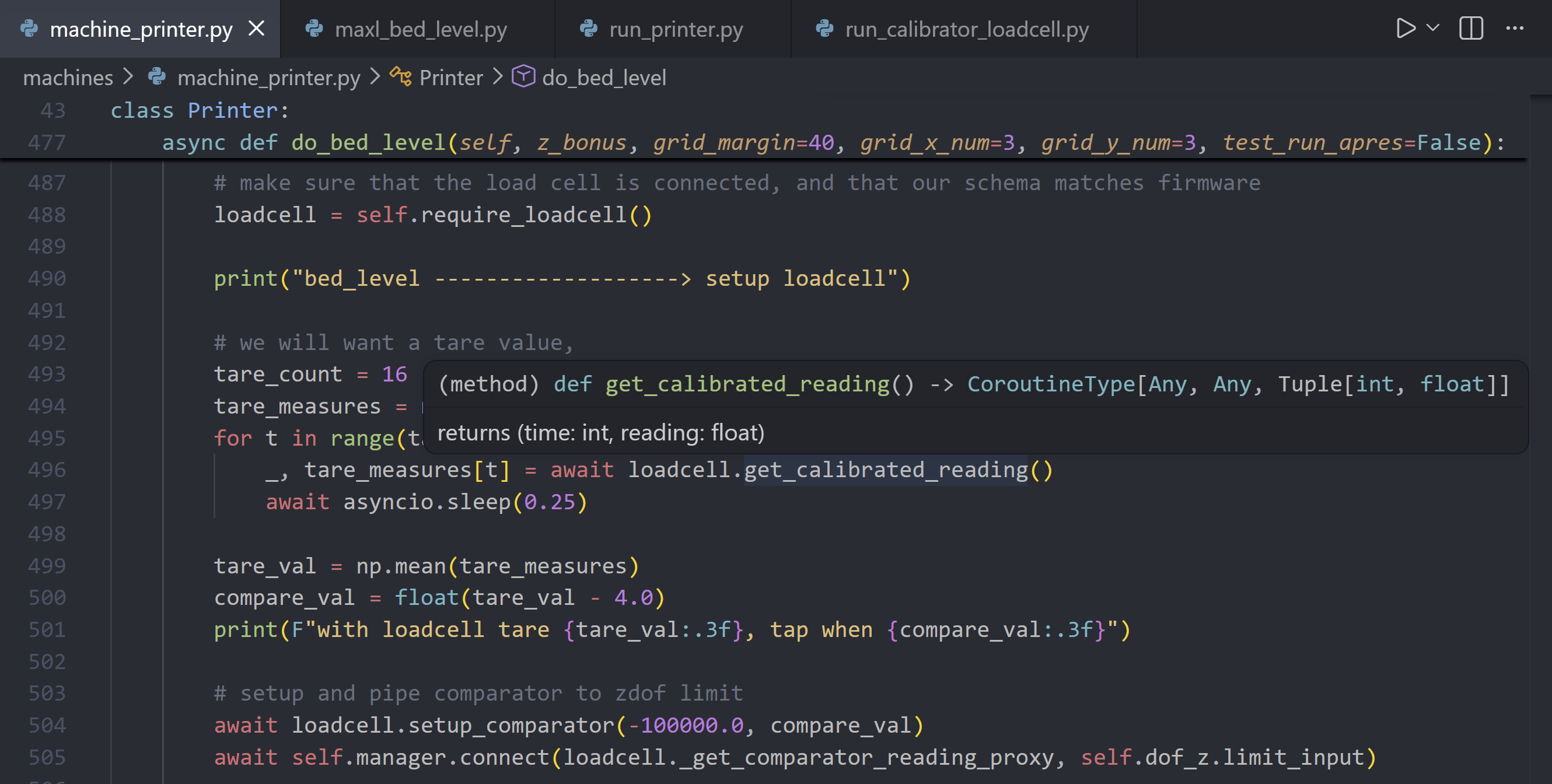
To level the bed, we can repurpose this homing routine to probe Z heights, and we can repurpose the load cell as an endstop switch. I show the block of code for the setup steps here in Figure 2.29, using a figure instead of a listing because I want to highlight a valuable property of the proxy system, which is that code is self documenting. Because each proxy contains type and output argument names, when they are used in modern IDEs (integrated development environments), their APIs can be auto-completed and inspected with e.g. the hover-over pop-up that is shown in that figure.
Also shown in Figure 2.29 is a call to self.require_loadcell() which ensures that the device is present before the next steps, and how RPC and graph operation is combined; first we collect a number of readings to tare the load cell, then we set up its internal comparator36 (both using RPCs), but connect it to the Z axis OneDOF block using manager.connect(). This effectively decouples parallel / asynchronous control (the switch state should trigger the OneDOF’s homing program to stop and turn around) from sequential control (iterating over an array of data points to sample and collecting each, as in Listing 2.32). Once the points are collected, the call is made to the leveller’s ._do_fit() method, and fit parameters are applied. The additional offset (the c parameter) is used to update the global height offset in the current machine state.
# in 'machines/printer.py'
class Printer:
    # ...
    async def do_bed_level(self, ...):
        # ...
        # now we can tap with the zdof home routine,
        async def z_tap(rate, backoff):
            # set stream up,
            await loadcell._get_comparator_reading_proxy.set_input_mode('timer', 250)
            tap_at = await self.dof_z.home(rate, backoff)
            # stop stream,
            await loadcell._get_calibrated_reading_proxy.set_input_mode('all_fresh')
            # return probe measurement,
            return tap_at
        # ...
        # probe at each,
        for p, pt in enumerate(z_pts):
            # go to position,
            self.dof_x.goto_pos(pt[0])
            self.dof_y.goto_pos(pt[1])
            await asyncio.gather(self.dof_x._wait(), self.dof_y._wait())
            # get val here,
            z_at = await z_tap(-1.0, 2.0)
            z_pts[p][2] = z_at
        # ...
But I mentioned that this also involves the time synchronization layer. The “MAXL Gap” (which can be tens of milliseconds, see Section 2.5.2) is between the OneDOF block that is generating points and the load cell’s readings; so comparator events appear in the past, but we need to know exactly where the Z axis was when the event occurred (not when the signal arrived). This constraint is why bed levelling routines must normally run within a GCode interpreter itself; they rely on centralized timing for this step.
Here, the OneDOF block receives a time-stamped switch state and uses that to query its local history of control points to ascertain where it was when the event occurred, i.e. interpolating along the spline defined by those points. The timing gap is still present and so in the interval between the switch trigger and the homing cycle’s update, some milliseconds pass with the machine still moving towards the endstop. In this case that means that the structure is being loaded against itself, which is permissible when the homing velocity is low enough — the motors can also be configured to use less torque in this step. The future work section of this chapter discusses how more of this logic could be re-located to improve this delay. But even in faster networked systems there will always be some timing delay between modules, so the approach here remains relevant.
Finally, we have the higher level interface. With GCode we would be writing down a new Gxx (although bed levelling itself is now semi-standardized at G32 [19]) and updating other scripts to reflect that. Here, we can simply add a new function to our machine.home() routine, or expose it as its own machine.do_bed_level(). Since those are defined in software, inspection and modification of function internals are much more straightforward.
2.7.4 Reconfiguration of Systems for Model-Building and Deployment
Same hardware, new software.
I mentioned in Section 2.7.2 how I use these tools to build systems-scale controllers from smaller components, e.g. with the load cell calibration and with motor modelling and encoder calibration routines. Since model building is so central to the thesis, I want to expand briefly and show especially the cases where not just individual devices or complete systems are used, but smaller sub-systems that lie somewhere in between those scales.
The most relevant sequence is in the motor— and then motion-modelling workflow. To calibrate motor encoders I use a small MAXL graph combining just a Timer block with a OneDOF block to drive the very lowest level of the motor’s controller (its voltage drivers) while sampling encoder readings and motor current measurements (see Section 4.4.0.1).
To model the motor I use a similar script, but now drive the motor directly using RPC calls that set drive current targets directly. I collect the same data from the motor, but now it is operating according to its own dynamics rather than following a MAXL spline. Using that time-series I can recover important motor parameters that relate its current readings to real torque values (see Section 4.5.1).
With a model for each motor, I can assemble machines to measure axes friction. In these tests most of the machine controller is assembled, except for the core velocity planner. Rather than driving it with a planner, I use MAXL’s chirp block to oscillate axes. Because kinematics are described separately from the planner itself, this can happen piecewise; for example in the 3D printers from Chapter 5, I can “chirp” the machine by driving its X and Y axes even though the motors are in A, B. I can also define separate tests for the X, Y half of the machine and the Z axes, which are kinematically separated. I describe that fitting process in Section 4.5.2.
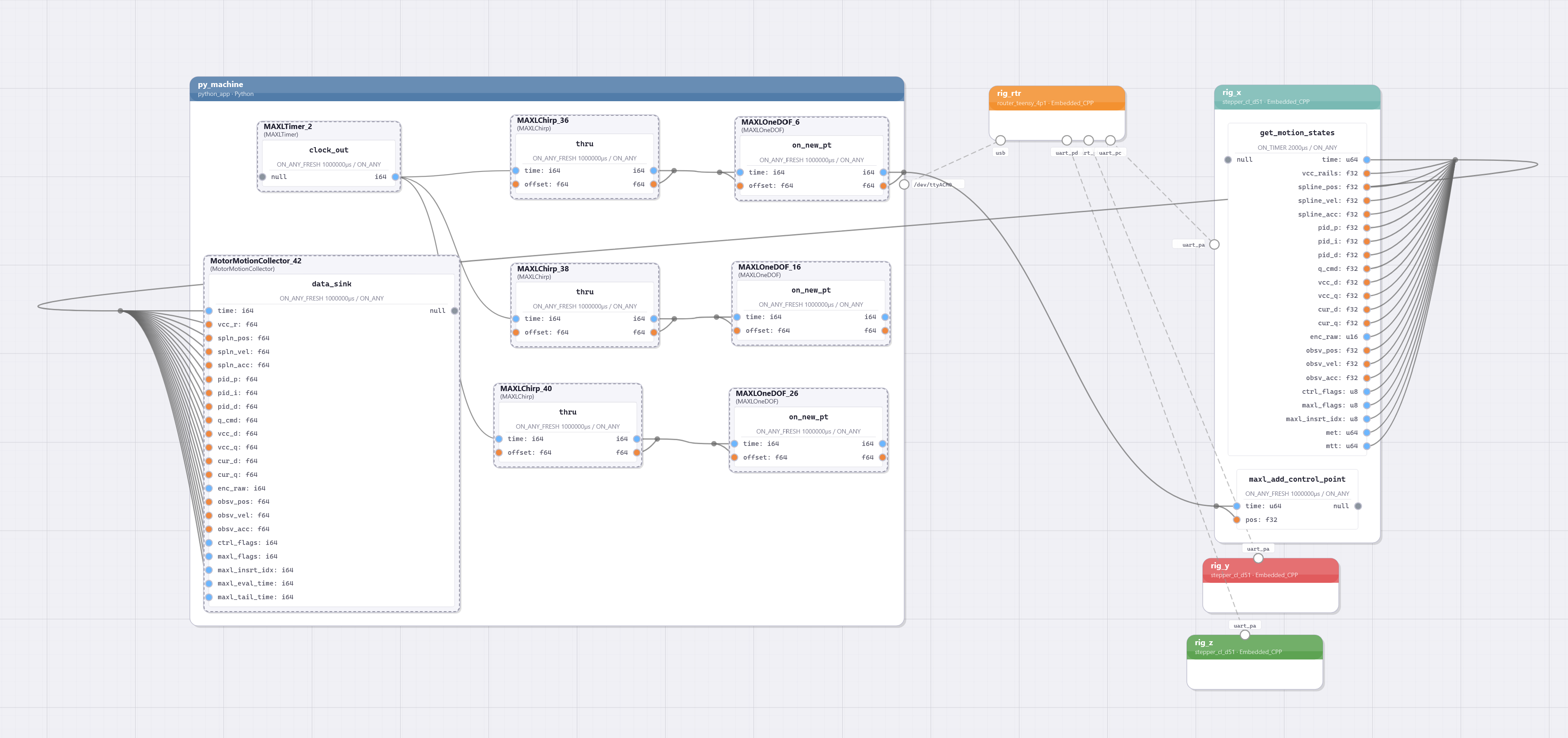
This method extends through to process modelling. In all, I use each printer in four total configurations across modelling and operation steps. Each of these run on the same hardware but using different configuration and tasking scripts:
- To run chirp tests on the XY/AB kinematic system.
- To run chirp tests through the Z motors.
- To fit flow models, where just the extruder system is activated. In this case, the motion control graph consists only of a Timer, a Chirp, and a OneDOF block (and the extruder motor). All other operation of the system (setting and waiting for nozzle temperatures) is done with RPCs, and data is collected with a series of Pipes: from the load cell, the extruder motor, and the nozzle heater.
- To operate the machine: using the full gamut of devices and adding the printer’s velocity planner interface.
Configurations of the CNC mill from Chapter 6 are similar, and I was able to build the machine and assemble these scripts in a few days because they didn’t require that I write any new MAXL blocks or firmwares, just modified scripts:
- To fit motion models, three configurations — one to test each axis.
- To run the machine, two configurations: one of which uses a trapezoidal planner, the other uses the optimization based planner from Section 4.6.
PIPES/MAXL also simplifies integration of the optimization based planners that I develop in Section 4.6 and 5.9 — I explain how they are connected to hardware via the frameworks in this chapter in 4.6.2, and Figure 2.31 renders one such PIPES integration (for the 3D printer, another system for the CNC machine is rendered in 4.11).
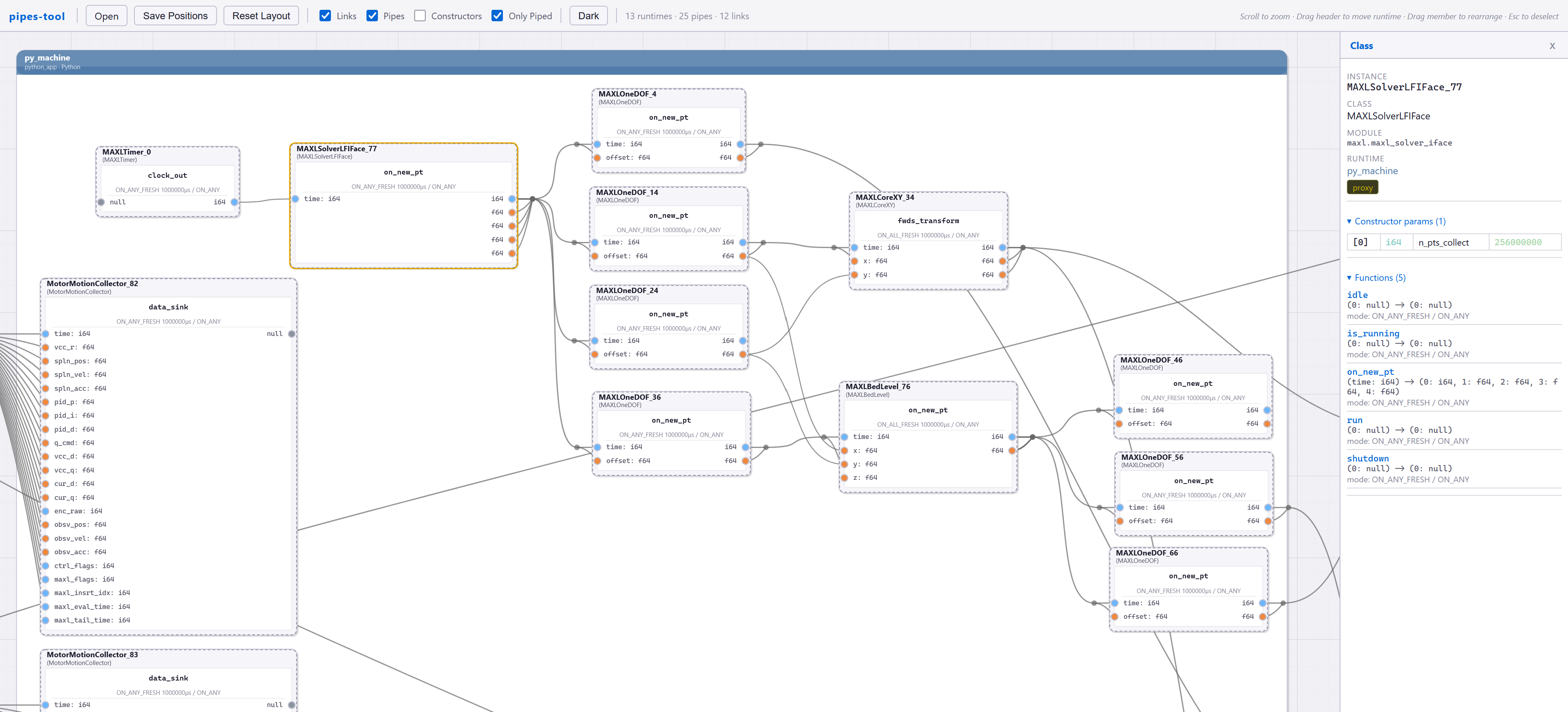
Because it is supported here by other MAXL blocks, the planner itself doesn’t need to manage auxiliary logic for things like axes homing, simpler kinematic transforms like bed levelling (whose effects have negligible ramifications for system dynamics), or any other control states and configurations: which motors are connected and how, their names, etc. Adding these features to the planner itself would be more cumbersome primarily because each implementation of the planner is (partially) unique to the machine it controls. But also because the planner runs in JIT-compiled code on the GPU (see Section 4.6) that is more difficult to inspect than vanilla Python blocks.
It also means that we can configure machines without the planner at all for each of the simpler routines that I just described. Because it is a module, we can swap it out entirely to test different types of velocity planner formulations on the same underlying hardware; I show results from an experiment that does so in Section 4.7.1. In that case the motion models that describe the system are still unifying; both planners make reference (one directly and one indirectly) to the same underlying physics.
Conversely, we can also disconnect the planner from hardware entirely and run it virtually, in which cases integration of “the rest” of the controller (homing, etc.) is not required at all; here we can simply drop those parts. If our models are well enough aligned this is nearly equivalent to running a simulation of the machine.
While the planner is less easily edited and inspected than most Python blocks due to its GPU deployment, it is more easily edited and inspected than the state-of-the-art model-based controllers for robotics that I survey in Section 4.2.7. Those are developed in a number of discrete steps and eventually compiled to run in hardware.
2.7.5 Reconfiguration of Modules for Machine-Building
Same software, new hardware.
So, the section above ran through a gamut of examples where we reconfigured software on top of the same underlying hardware, but I also have some examples of the opposite situation: variable hardware with re-use of software components. This in itself is not novel because most GCode interpreters can be reconfigured for different machines, but the range of machines is worth showing and the reconfiguration strategy is quite different.
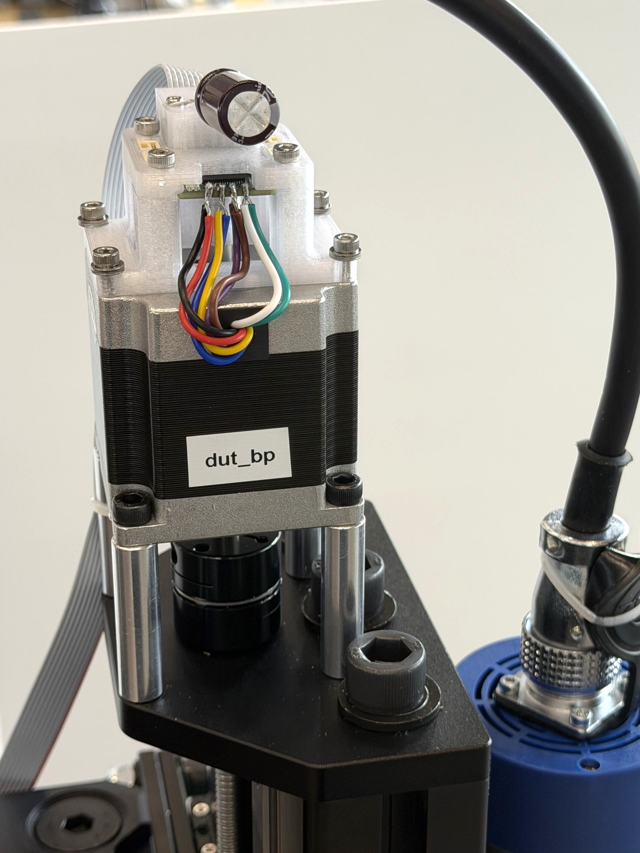
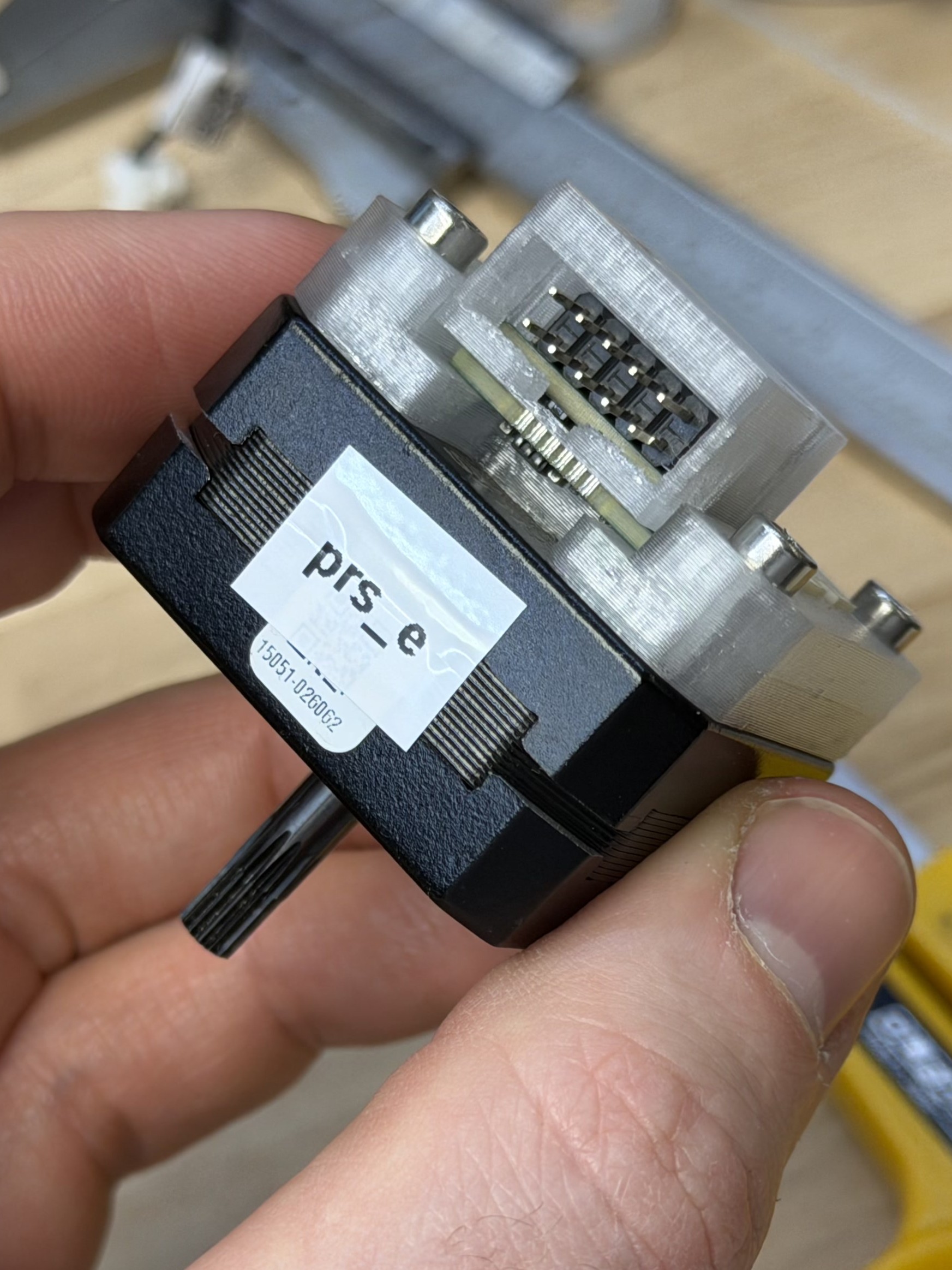
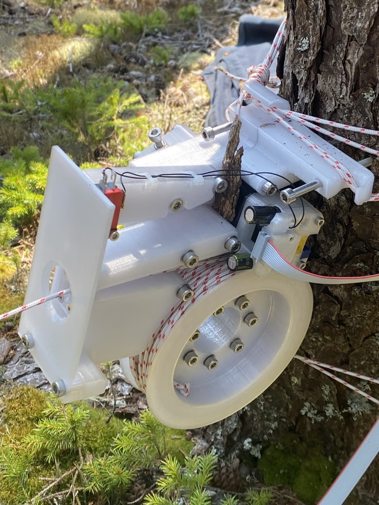
In terms of core components, the OneDOF module is repeated by far the most often in different systems and configurations, which makes sense given that most machines have at least one degree of freedom. Its utility in quickly adding simple control interfaces for “the rest” of machine control (e.g. jogging, homing, etc) is invaluable.
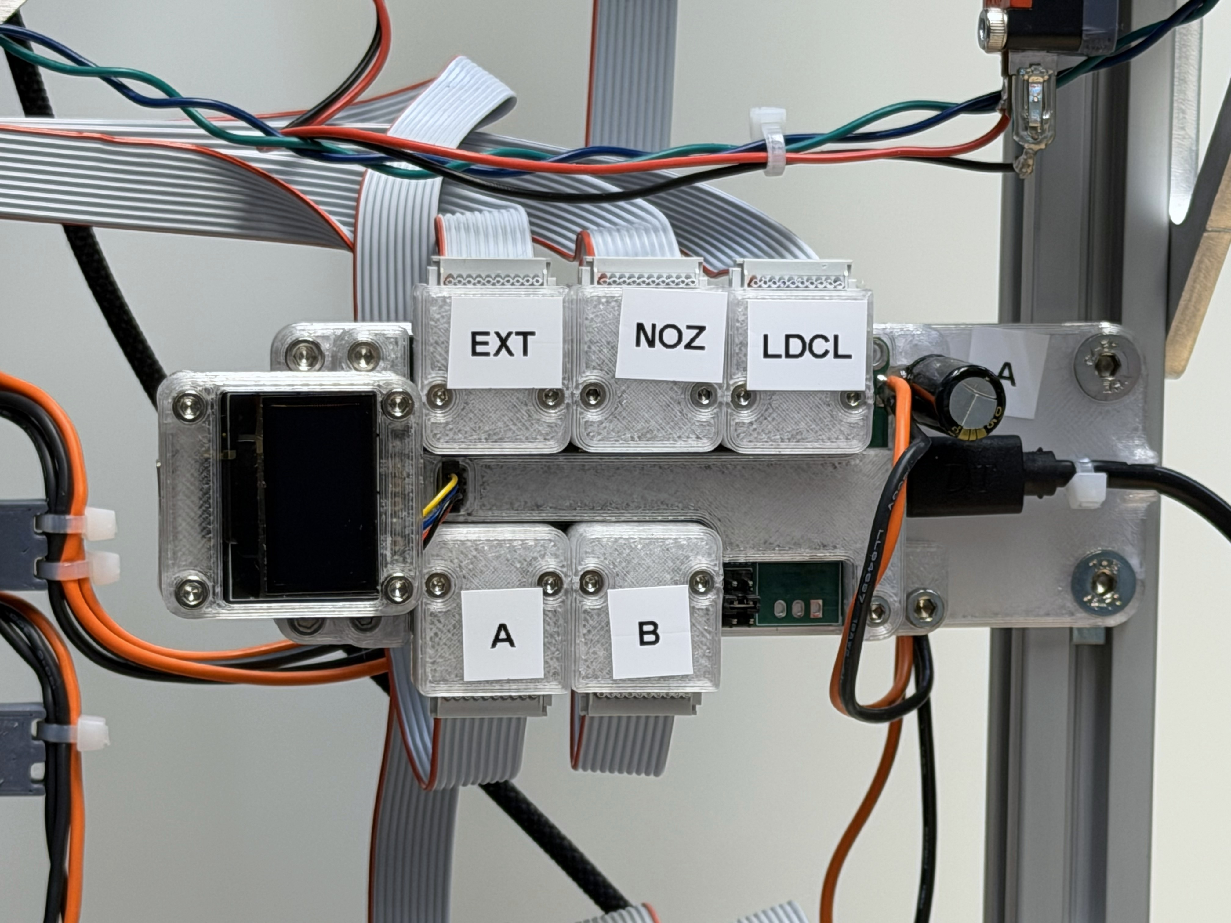
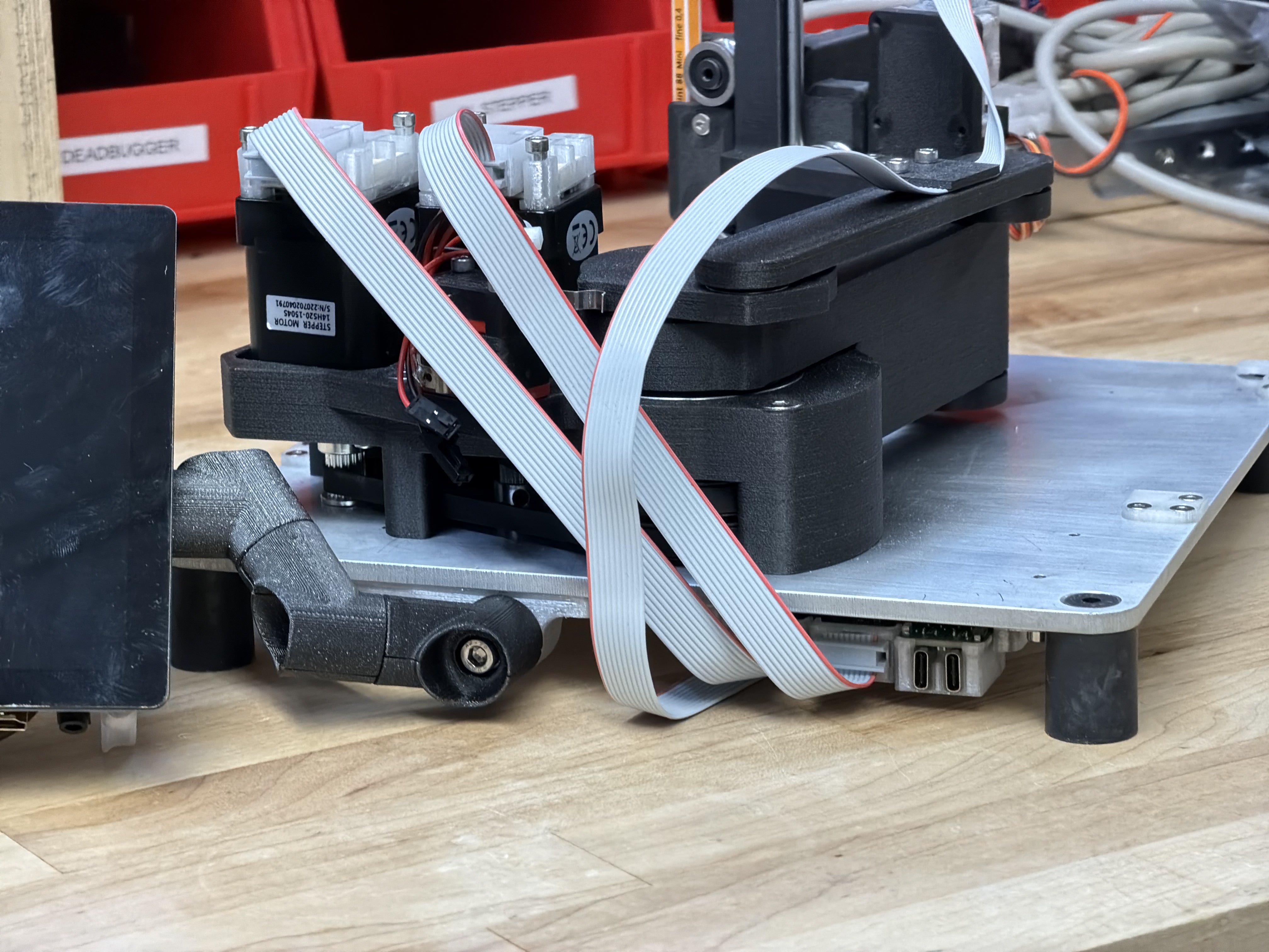
This has a limit though, for example the velocity planners for the 3D printer and CNC mill are each unique: they are “reconfigured” for each machine by re-writing software. In kinematics this is true as well, we cannot compose arbitrary mathematics with the existing set of MAXL blocks, and need a new module each time we encounter some new arrangement of axes.
2.7.5.1 Reconfiguration Across Variable Kinematics
When we do encounter new kinematics, authoring new MAXL blocks to suit is easier because they are written in Python and declaring that a generic Python class should be interpreted as a Pipes Class is straightforward: we just add the @pipes_class_implementer class decorator, as I showed in Listing 2.20. That again reduces the problem to just the one new class definition. The same is true of many other machine control systems, i.e. Klipper [92], Duet (on the RepRapFirmware [18]) and Smoothieware [141] can add kinematics in a similar manner, but in each of those cases they are defined in firmware that is then recompiled. StepDance [95] makes great strides in terms of modular kinematic descriptions and actually uses a similar strategy to this one, but is also firmware-defined and provides limited interfaces out of embedded devices (see Section 2.2.4.6).
During MAXL’s development I helped to host a workshop at the CBA where participants developed drawing machines. I participated as a machine control enabler and used MAXL and OSAP to quickly develop controllers and kinematics models for each of these machines. That involved working with machine designers to describe their kinematics as functions that map tool-tip positions to motor positions (inverse kinematics or IK functions), and then authoring those together as Python functions. Those were then written as MAXL blocks, and connected to hardware with an early version of PIPES. We successfully drew .svg files with each machine. The machines from the workshop are in Figure 2.34. Two MAXL blocks were developed then that were also re-used or based on re-use; I re-used the Scara kinematics block in the “Little Guy” machine which I built after the workshop (it is pictured in Figure 2.33) and the Kaos kinematics block required only a slight modification to the CoreXY block.
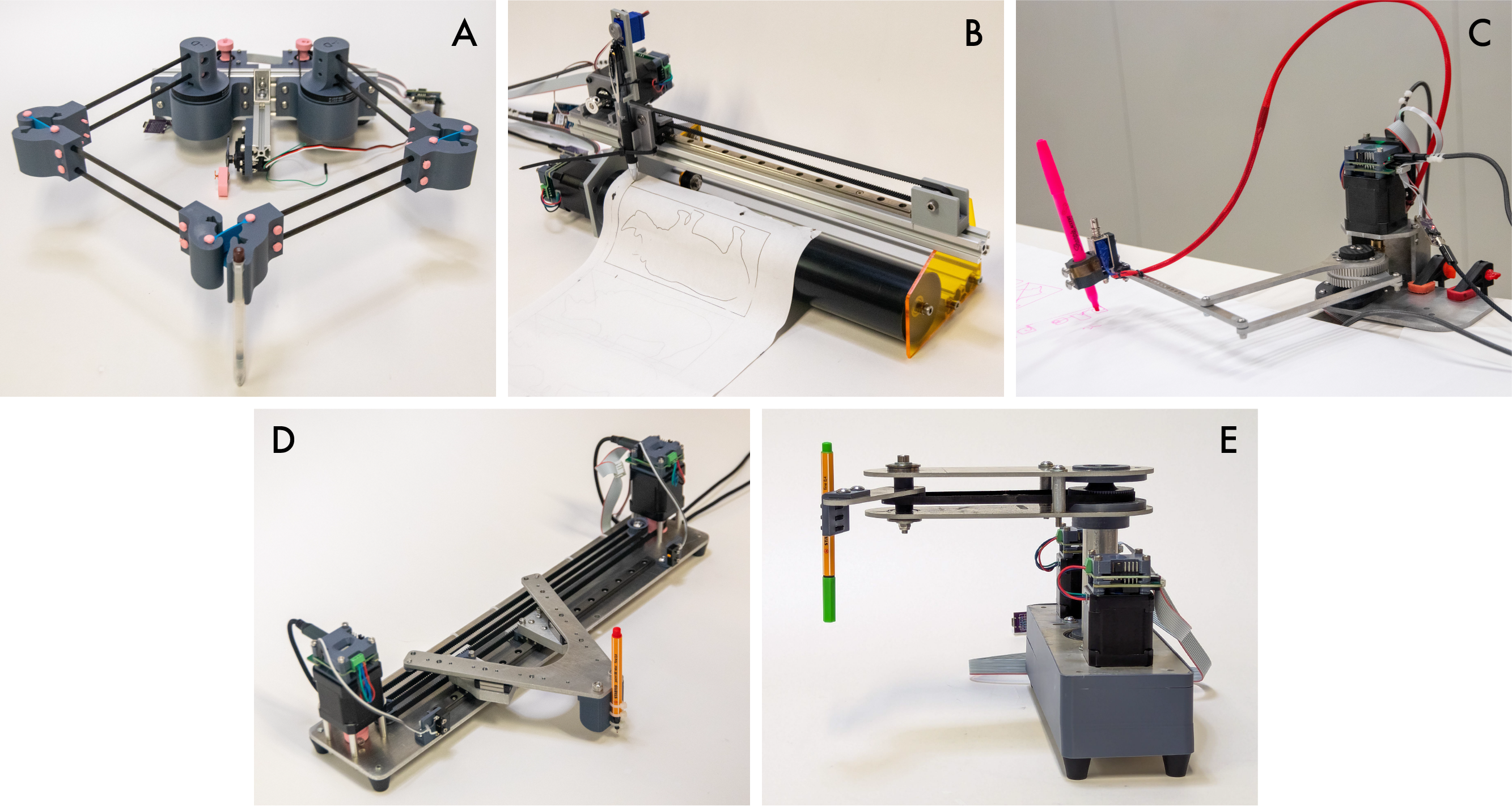
2.7.6 Visibility of Internal Control States
Most velocity planners are in firmware, beneath GCode, so we cannot see the results of their internal operation. MAXL and PIPES go to some length to remove velocity controllers from firmware, relocating them as software objects. One of the primary benefits of this is the simple utility of being able to inspect these controllers’ outputs and easily modify them. Their configurations and those configurations’ relationship to our machine hardware and our target path geometries can combine to produce interesting results.
For the first example of this, see Figure 1.7 from the introduction, where I show that in some parts of path- and machine-parameter space, the feed rates that GCodes specify may never be reached when they are actually run on hardware.
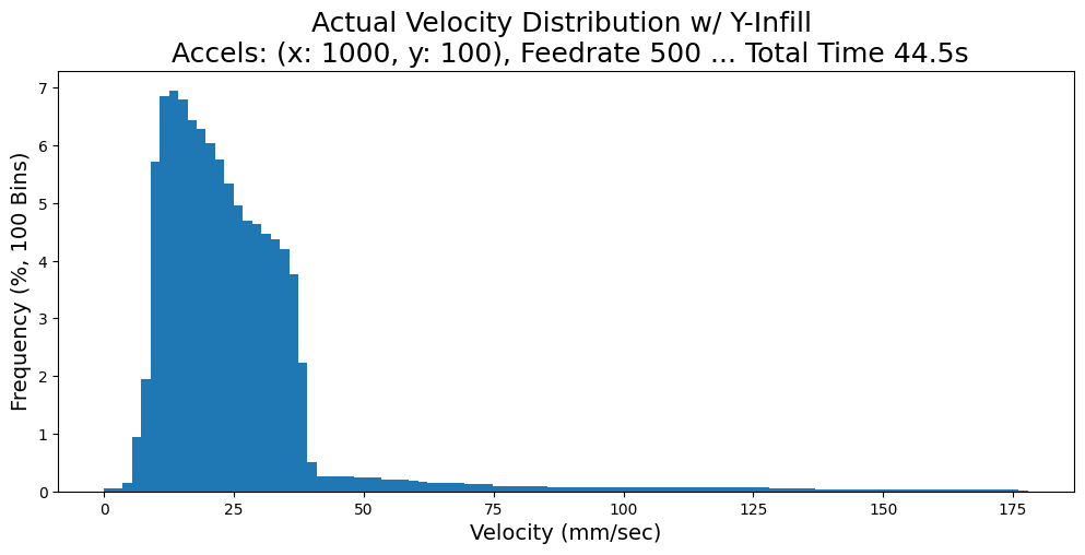
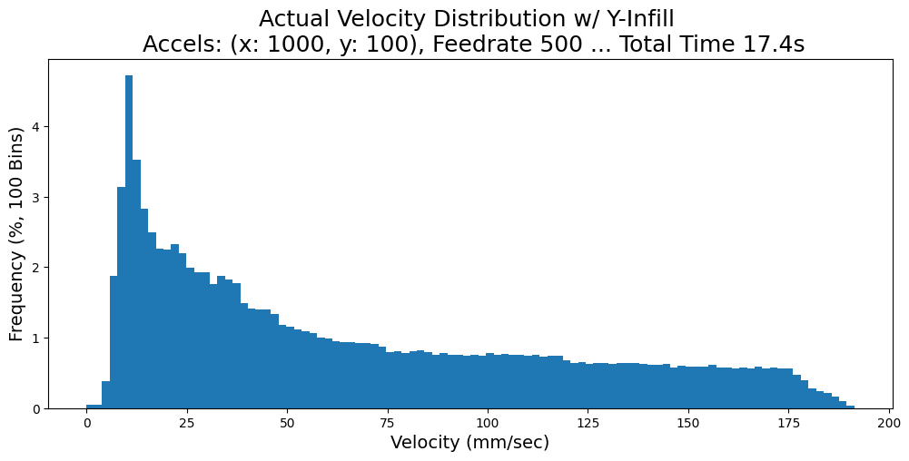
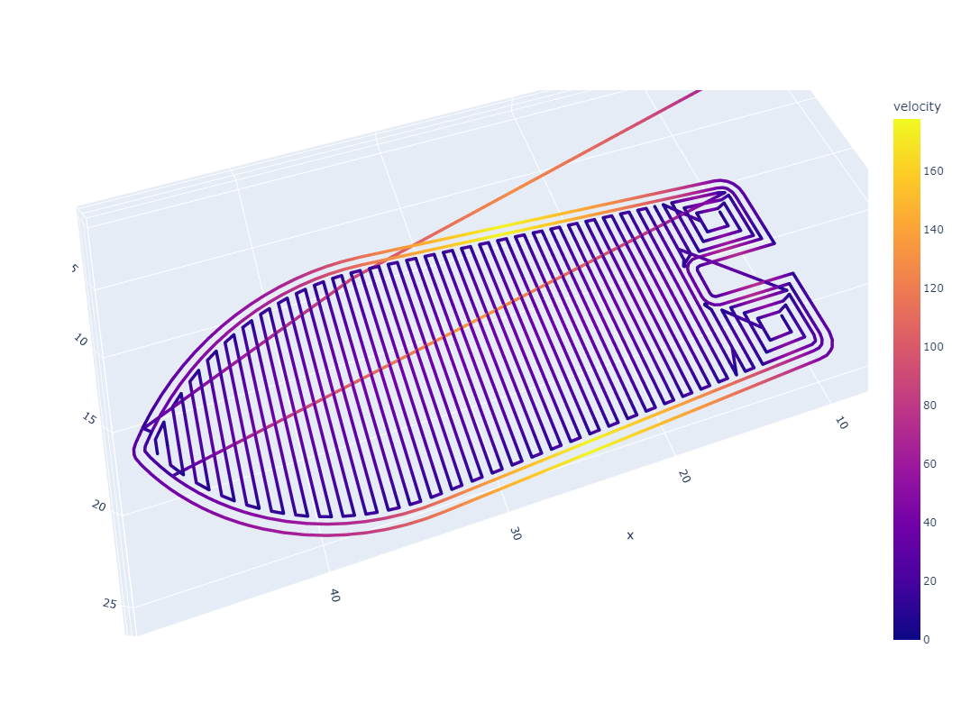
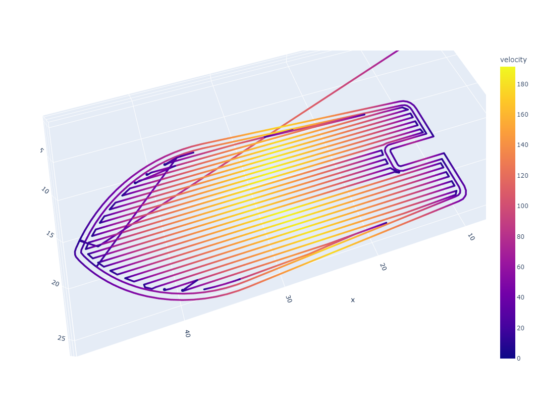
For another example here, we can consider CoreXY ([122] Section 2.5.4.6): machines with this layout have highly anisotropic dynamics. Both motors work together to move the machine in X and in Y, but the moving mass in X (just the end effector) is significantly lower than that in Y (which includes the end effector along with the y-beam). In the figure below, I show outputs using a trapezoidal planner which deploys 10x more acceleration in the X axis than in the Y; we can see that changes to path geometry (like aligning repeated, long line segments to the motion systems’ anisotropy) can significantly change outcomes (like total processing time, and actual processing feed rates). Exposing these results to machine users and builders could help them better understand why their machines behave in unexpected ways.
In Section 6.3.1, I show how this result from MAXL’s structure enables the development of a simple tool for visualizing chip load deviation in CNC machining toolpaths. In that context, this knowledge can be invaluable before a path plan is run on a machine because significant chip load deviation can lead to chip welding (rather than cutting). The next section describes how this method is extended to more easily map sensor readings back onto trajectories, which is valuable when we want to make process measurements as our machine is running.
2.7.7 Time Synchronized Sensing and Data Collection
Using a time basis for trajectory representation leads to many other outputs in this thesis, because it allows us to combine sensor data with motion data. I show how this capability is used for model building in:
- Fitting kinematic models, Section 4.5.2
- Improving kinematic models using data generated during machine operation, Section 4.7.3
- Fitting dynamic extruder parameters, Section 5.5.3
- Fitting coupling terms between extruder motors and melt flow models, Section 5.6
In each of those cases, I use motion controller inputs to drive systems while collecting time-series data of motion states alongside sensor data, which are then used to fit (or update) models. I also show how this capability is used to evaluate motion systems:
- To evaluate the quality of kinematic models, Section 4.7.2
- To generate new insights from 3D printer data that combines sensor, motion, and planner states, Section 5.11.1
- To make cutting force estimates, combining kinematic models, motor models, motor data, and trajectory data, Section 6.4.4
Piped connections are useful here because we can configure remote functions to send data back to our configuration and control scripts in a timely manner. That involves making connections up through the network using manager.connect() and then configuring each function’s input mode to run at a defined interval. Developing data collection in this way means that the Python script itself doesn’t have to repeatedly poll devices, which would introduce extra jitter in data samples. The transmission intervals can also be tuned according to network performance and data resolution priority, and of course sensor readings are all time stamped against their local device’s estimate of system time (from Section 2.3.2.2).
2.7.8 Enabling the Application of Large Compute in Machine Control
Connecting high-powered computing systems to machine hardware is often difficult because operating systems can be nondeterministic and networks that span between them introduce lag. I discussed this in some detail in the background section to this chapter, and made direct comparison between this systems architecture and model-based controllers that have been developed by other researchers in Section 2.6.2.
I described in Section 2.5.2 how we can introduce a fixed-size, fixed-interval timing gap between these layers to approximate deterministic operation across this layer. This is what allowed me to deploy the GPU-based velocity planner from Chapter 4 and 5, which requires substantial computing power.
However, the method is also somewhat limited. As I will discuss in Section 4.6.2, I had to develop an additional separation between the OSAP runtime that controls the machine in Python and the planner code itself. Although also written in Python, the planner blocks Python’s asyncio loop while it generates new solutions, which can take up to 100 milliseconds. PIPES is designed with parallelism in mind, but OSAP relies on cooperative scheduling and while the planner is working the rest of the system (that is collecting data and transmitting control points from prior solution components through a PIPES graph), needs to keep running. I discuss how OSAP could be improved to support this more natively in Section 2.9.
Introducing that timing gap does not come for free; the gap is configured against the worst case network and computing delay between the operating system and remote devices. To understand how we can configure the gap intelligently, and to see how much of a gap is really required, we have the next section on timing.
2.7.9 Timing Performance Analysis
I’ve mentioned in a number of places how network and compute performance can constrain machine performance. The OSAP runtime, PIPES architecture and MAXL framework are each designed with this in mind, favoring simple low-level operation that that can be computed quickly but adding a slower global configuration step to combine that with flexible development. I also discussed the trade-offs between flexibility and overhead; adding layers and abstraction tends to require additional overhead.
In this section I first make a broad timing comparison between the model-based machines that I developed in OSAP / PIPES and MAXL and other researcher’s efforts, and then work through packet size overhead, underlying timing performance using measurements from the clock synchronization tests, and finally relay how those relate to overall bandwidths / performance of these systems.
2.7.9.1 Timing Comparison to Related Model-Based Control Research
In Section 2.6.2 I looked at two other researchers’ efforts to deploy model-based control for machine systems (both CNC milling centers). I already discussed how those differ at an integration level, but a timing comparison is worthwhile as well; one of them (Ward [137]) collects readings at \(250\text{Hz}\) and issues new control outputs at \(100\text{Hz}\) and the other (Tong [139]) does both at \(100\text{Hz}\). Both integrate over heterogeneous networks (including IP-based links, fieldbusses and even analog links) that are manually configured to bridge between realtime control components and higher power workstation computing where models are deployed.
The controllers that I build with the systems in this chapter collect data from actuators at \(500\text{Hz}\) and transmit new control points at \(250\text{Hz}\). The actuator data includes more motion derivatives and internal current controller states than Ward and Tong collect, a full list of these is listed in Section 4.4.1. I collect data from the 3D printer load cells at \(150\text{Hz}\), and temperature sensors at only \(30\text{Hz}\), see Section 5.4.2. The basis spline control points that I send through MAXL are delivered directly to interpolating motors and can be evaluated for position, velocity, and acceleration values. Ward and Tong’s systems both connect model-based controllers to their machine’s internal feed rate override handle, which adds more and somewhat unpredictable delay between updated commands and real response from hardware; their machine’s hidden velocity planner uses the feed rate override as a reference signal that it subsequently tracks. In fact this signal is indirect in another way because it modifies the target feed rate that is written into the GCode that their machines and model-based controllers are simultaneously consuming.
I was surprised to see these relatively low bandwidths. It is hard to tell if these authors are limited by their model’s complexity and computing (both build substantial control algorithms) or by their networks, network bridges, or by the machine interpolators. It seems as though even if the controller’s predictive bandwidth were limiting they would have preferred higher bandwidth input data if it were available to improve measurement resolution. That said, they may have identified that their system’s dynamics were not themselves much faster than \(100\text{Hz}\) — these are bigger machines with larger time constants than the ones that I have instrumented.
2.7.9.2 Packet Size Overhead
I’ve collected a few key messages and calculated packet overhead for each across PIPES and OSAP in Table 2.6. OSAP header bytes (second column), include a baseline of six bytes for each packet’s instruction pointer, maximum transmission unit, time to live, and (after the route) the transport protocol type. Headers are variable length because routes can include multiple instructions; one byte for each link gateway traversed, two for each fieldbus gateway traversed, and three bytes to encode the source and destination ports; see Table 2.4 for more details on the OSAP routing system.
The third column counts bytes in the raw data that is transmitted in each message, i.e. the size of the message data in CPU memory. PIPES bytes (fourth column) accounts for bytes used to encode the argument mapping (which values will be delivered to which input arguments of the receiving function) and each value carries its own type byte so that the receiving function can check against its signature and convert (or reject) data where necessary; see Table 2.5. For each PIPES message, there is a one-byte key, one-byte count of arguments, and each argument requires two additional bytes (one to map, one to type); so we have \(2 + 2n\) bytes of overhead for each where \(n\) is the number of arguments. PIPES overhead (fifth row) is the share of application layer bytes that are used for this mapping / typing encoding. There is substantial overhead here, but the encoding removes state from PIPES connections. We may be able to have both, as I briefly discuss in Section 2.9.2.2.
Total overhead is calculated as the percentage of each packet that is used for OSAP and PIPES operation. Small packets along long routes (e.g. in the third row) are the most punishing in this regard, and overhead is smaller for larger packets. For a brief comparison to IP-based networks, the IPv4 packet header is 16 bytes long and IPv6 header is 40 bytes. These are normally wrapped in Ethernet frames for another 38 bytes of overhead.
So, in an IPV4 network over Ethernet the packet in the third row (at \(62.5\%\) total overhead with OSAP) would include \(83.3\%\) networking overhead. Over IPv6, \(87.5\%\) (this is still including the PIPES overhead). At the same time, Ethernet’s bitrate is much faster than the simpler embedded networks I use in these examples to compute wire times (which are explained shortly) so, while larger, IP/Ethernet frames would move faster. That said, Ethernet baud rates require Ethernet-capable devices to read them and there is a natural correlation between a microcontroller’s processing power and its ability to manage extremely high data rate networking. In Section 3.4 I explain in some more detail why I prefer simpler (slower) link layers for these systems.
| Message | OSAP Header | Raw Data | PIPES Map and Types | PIPES Overhead | Total Overhead | Wire Timee A | Wire Timef B |
|---|---|---|---|---|---|---|---|
| \(\text{Bytes}\) | \(\text{Bytes}\) | \(\text{Bytes}\) | \(\%\) | \(\%\) | \(\mu\mathrm{s}\) | \(\mu\mathrm{s}\) | |
| MAXL Control Pointa | 10 | 12 | 6 | \(33.3\) | \(57.1\) | \(224\) | \(107\) |
| MAXL Control Pointb | 11 | 12 | 6 | \(33.3\) | \(58.6\) | \(232\) | \(110\) |
| MAXL Control Pointc | 14 | 12 | 6 | \(33.3\) | \(62.5\) | \(256\) | \(120\) |
| Motor Motion Dataa | 11 | 42 | 24 | \(36.4\) | \(45.5\) | \(616\) | \(270\) |
| Motor Modelling Dataa | 11 | 93 | 46 | \(33.1\) | \(38.0\) | \(1200\) | \(513\) |
| Load Cell Dataa | 11 | 12 | 6 | \(33.3\) | \(58.6\) | \(232\) | \(110\) |
| Heater Dataa | 11 | 16 | 8 | \(33.3\) | \(54.3\) | \(280\) | \(130\) |
| Time Config Query Responsea,d | 11 | 65 | n/a | n/a | \(14.5\) | \(608\) | \(267\) |
a Routed across one link gateway.
b Routed across two link gateways.
c Routed across three link gateways and one fieldbus gateway.
d The time configuration query response is made through OSAP’s native model-view controller; data is packed according to a pre-defined schema and so there is no PIPES overhead in this case.
e At \(1000 \text{Kbps}\).
f At \(3000 \text{Kbps}\) through a UART link including COBS packet encapsulation and CRC16 error checking.
For example MAXL control points contain two values: a timestamp (a 64 bit / 8 byte wide integer) and a floating point value (32 bits). The motor motion data and motor modelling data sets are in Tables 4.3 and 4.4. The timing configuration packet (last row) is unique to this set in that it is not part of the PIPES system, it is one of the OSAP model-view controller messages. This is not the message that is used to synchronize clocks, it is the message used to inspect clocks.
I also include two “wire time” values, these show how long it takes to transmit each message on network links under two conditions: the first is a generic \(1000 \text{Kbps}\) link and the second is a \(3000 \text{Kbps}\) UART link (where each byte adds a start and stop bit) that includes COBS packet delineation and CRC16 error detection; this is the type of link that I used most often to connect devices to one another across OSAP.
2.7.9.3 Timing Analysis with Clock Synchronization Data
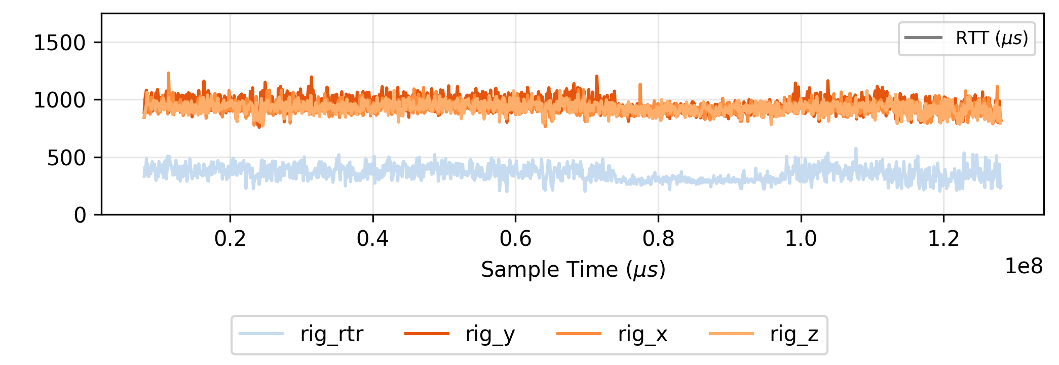
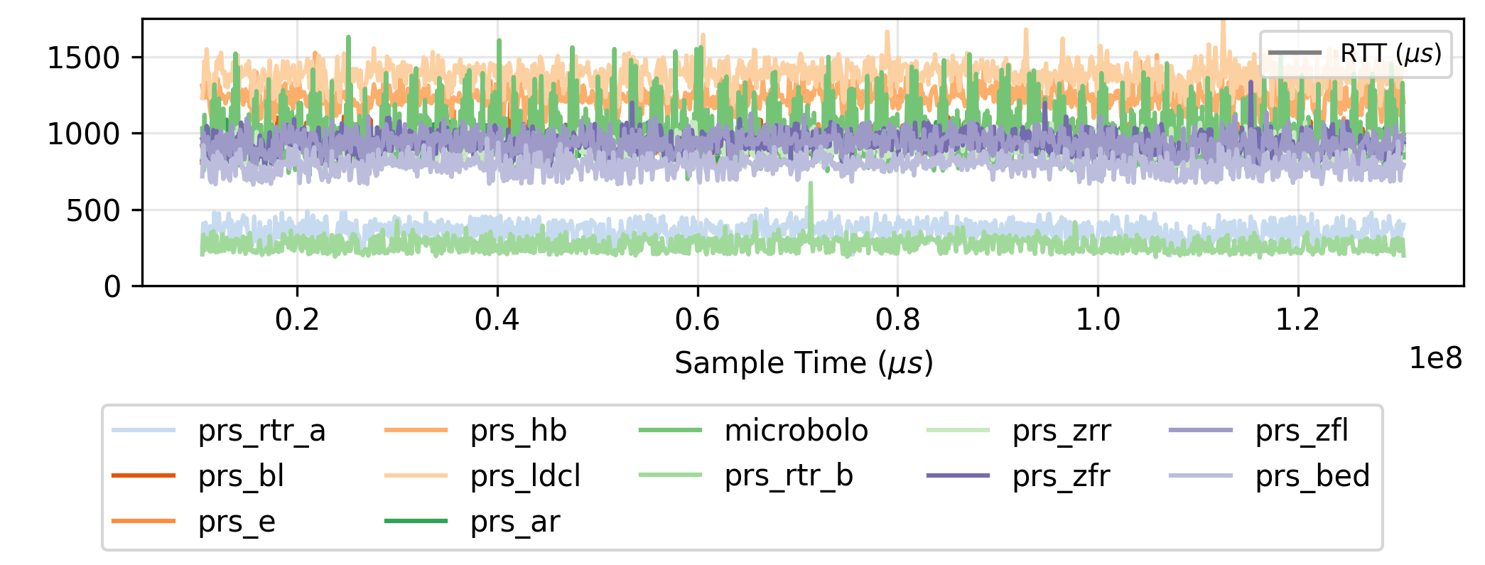
So, that covers packet overhead and wire time gives us an estimate of the network layer’s underlying performance, but time is also consumed processing messages within the OSAP runtime. Because OSAP uses software defined links, some processing time is also required to e.g. delineate packets and process CRC in each (depending on the link gateway).
To make an estimate of how much time is used in these processing steps, we can look at data from the time synchronization tests (Section 2.3.2.2). Figure 2.38 shows round trip times measured between a Python script and each device in the milling machine from Chapter 6 and the FrankenPrusa from Chapter 5. In these tests a Python script queries all the remote OSAP runtimes that it discovers using the MVC “Get Time Controller Configuration” message, which is one of the messages in Table 2.6 above. This returns data that is useful to analyze how each device’s clock synchronization routine is working, but here we are just using the round trip times (RTTs) for each message, which is simply measured in the Python script. Otherwise, the message load itself does well to approximate all the steps that a runtime manages when it receives any other message: add the packet to the runtime’s stack, handle it in the main loop, pull some data out of memory and perform some calculations, and then reverse the route and issue the reply. This message does not go through the PIPES system, but it does use the same data serialization routines that PIPES uses. Each query response is 76 bytes long (including the packet header and the message key) with two uint64 values, one uint32 value and eleven floating point values.
To work out which part of each message’s total RTT is taken up by the runtime’s processing steps (which represents computing overhead) rather than the underlying network link delay, we can remove each packet’s wire time (each RTT includes a trip up and back down the wire). For the devices that are connected immediately to the Python runtime (first three rows of Table 2.7, where results here are displayed), the measured processing time includes both the device processing time and the Python processing time. Based on the fact that one of these devices (the microbolometer) shows a processing time much greater than the other two indicates that the Python processing time must be below ~ \(250 \mu\mathrm{s}\). For other devices, we remove from their RTT the mean RTT of the intermediate device. This is presuming that the intermediate RTT accounts for both the upstream wire time and also the Python runtime and the intermediate device’s processing time to passing the message on. This is somewhat lossy because passing the message is probably faster than handling the message, but it should get us in the right ballpark. In Section 2.9.1.3, I explore how OSAP could change in order to make this type of timing analysis more straightforward, as it turns out to be an incredibly valuable systems assembly tool.
| Device | Devices and Links in Route | Closest Link Wire Time | RTT Mean | RTT \(\sigma\) | Max RTT \(99.99\%\) | Processing Time Est. |
|---|---|---|---|---|---|---|
| \(\mu\mathrm{s}\) | \(\mu\mathrm{s}\) | \(\mu\mathrm{s}\) | \(\mu\mathrm{s}\) | \(\mu\mathrm{s}\) | ||
| Message Hub Aa | USB 2.0 HS (CDC) | \(3.2\) | \(350.0\) | \(64.0\) | \(541.9\) | \(346.8\)f |
| Message Hub Ba | USB 2.0 HS (CDC) | \(3.2\) | \(264.7\) | \(48.4\) | \(580.6\) | \(261.5\)f |
| Microbolometerb | USB 2.0 FS (CDC) | \(32\) | \(979.3\) | \(185.8\) | \(1843.6\) | \(947.3\)f |
| Bed Heaterc | Hub B + UART | \(534\) | \(822.9\) | \(58.3\) | \(963.3\) | \(24.2\)g |
| Extruder Motord | Hub A + UART | \(534\) | \(920.0\) | \(59.1\) | \(1170.6\) | \(36.0\)g |
| B Motord | Hub A + UART | \(534\) | \(951.6\) | \(68.1\) | \(1246.5\) | \(67.6\)g |
| A Motord | Hub A + UART | \(534\) | \(947.8\) | \(66.0\) | \(1155.7\) | \(63.8\)g |
| Z Motord (Rear) | Hub B + UART | \(534\) | \(890.9\) | \(68.2\) | \(1126.5\) | \(92.2\)g |
| Z Motord (Right) | Hub B + UART | \(534\) | \(917.9\) | \(71.4\) | \(1166.7\) | \(119.2\)g |
| Z Motord (Left) | Hub B + UART | \(534\) | \(920.2\) | \(71.1\) | \(1140.7\) | \(121.5\)g |
| Extruder Heatere | Hub A + UART | \(534\) | \(1217.3\) | \(68.4\) | \(1567.1\) | \(333.3\)g |
| Load Celle | Hub A + UART | \(534\) | \(1358.9\) | \(83.3\) | \(2033.4\) | \(474.9\)g |
a NXP i.MX RT1062 at \(600\text{MHz}\).
b Raspberry Pi RP2350 at \(266\text{MHz}\).
c Raspberry Pi RP2040 at \(200\text{MHz}\).
d Atmel ATSAMD51 at \(180\text{MHz}\).
e Atmel ATSAMD21 at \(48\text{MHz}\).
f This includes processing time in the endpoint device (one step) and in Python (two steps: generating the query and receiving the response).
g Calculated by removing the mean RTT of the intermediate device (Hub A or B) from the mean RTT of this device, and also removing the closest link wire time.
2.7.9.4 Timing the MAXL Gap
So, with a better understanding of the packet and runtime overheads, we can reflect those onto relevant timing and bandwidth characteristics for MAXL. Earlier I compared data rates between the systems in this thesis and two other researchers efforts to also build model-based machine controllers, showing that data collection in this case is faster than their implementations. Again it is hard to know if their timings are based on systems dynamics or network / systems performance limits.
That said, MAXL also inserts a gap (see Section 2.5.2) between the trajectory source (in Python on an operating system) and sinks (embedded devices). This can be as wide as \(128 ms\) \((7.8 \text{Hz})\) or as short as \(~ 2.048 ms\) \((488.3 \text{Hz})\) depending on the underlying networks and the tolerance for occasional errors that arise from the operating system’s indeterminacy. Really there is no lower limit in the framework; the value I presented just now is based on an optimistic estimate on best-case computing delays if e.g. we ran all of a system’s actuators on high speed links and devices a-la the first two rows of Table 2.7 above.
To quantify this gap, I have Table 2.8. It shows a range of intervals and network / operating systems gaps; these are configurable according to overall system performance. I have discussed how network feedback and inspection tools could be used to configure each gap in order to minimize overall delay, and how PIPES / OSAP enables reflection between program configuration and networking; source routes are configured alongside program wiring and data in the network is typed and inspectable. See Section 2.8.5 for more on that topic.
The second column of the table shows bandwidth required to transmit MAXL control points to four actuators across a range of interval sizes (in Kilobits per second \(\text{Kbps}\)). That is calculated for packets sent across two link gateways through OSAP and PIPES, including argument type maps etc.; see Table 2.4 for the OSAP packet header (11 bytes in this case) and Table 2.5 for the PIPES data encapsulation and argument mapping (18 bytes for each MAXL control point via PIPES).
The third column of the table is the gap required for safe interpolation of control points according to the interval; each spline interpolator needs at least three points in the future to be loaded in memory in order to compute the basis spline’s values.
The last two columns are resulting bandwidths in \(\text{Hz}\). The first is for feed forward responsiveness between trajectory generation and arrival at interpolators and the second is for round-trip cycles in feedback systems. This includes total delay between sensor sampling and return of that data through the network under worst case operation, computation of new trajectories and finally their interpolation in hardware.
| Interval | Data Rate | Spline Interval Gap | Net / OS Gap | Feed Forward | Round Trip |
|---|---|---|---|---|---|
| \(\text{ms}\) | \(\text{Kbps}\) | \(\text{ms}\) | \(\text{ms}\) | \(\text{Hz}\) | \(\text{Hz}\) |
| \(16.384\) | \(57\) | \(49.15\) | \(98.3\)e | \(6.8\) | \(4.1\) |
| \(4.096\) | \(227\) | \(12.29\) | \(49.2\)a | \(16.3\) | \(9.0\) |
| \(4.096\) | \(227\) | \(12.29\) | \(4.1\)b | \(61.0\) | \(48.8\) |
| \(4.096\) | \(227\) | \(12.29\) | \(32.8\)c | \(22.2\) | \(12.8\) |
| \(4.096\) | \(227\) | \(12.29\) | \(4.1\)d | \(61.0\) | \(48.8\) |
| \(1.024\) | \(906\) | \(3.072\) | \(1.0\)f | \(244.1\) | \(195.3\) |
| \(0.512\) | \(1813\) | \(1.536\) | \(1.0\)f | \(390.6\) | \(279.0\) |
a,c These are the configurations I used for the FrankenPrusa and milling machine.
b,d These are the fastest possible configurations for either, supposing we limit the network / OS gap to approximately 2x the worst case RTT as measured in the time synchronization tests.
e This is representative of very slow, non-deterministic networks, e.g. using simple wireless links. While this is obviously not responsive, the loose spline interval reduces the data rate significantly and clock synchronization would still enable co-ordinated motion.
f These are representative of two configurations for a system that runs e.g. entirely on the high-power microcontrollers that I used for the Hub / Message passing devices; Table 2.7 shows that their maximum RTT is only around \(600\mu\mathrm{s}\) on the safe side. Getting the message down to the device takes only half of the RTT.
In practice, I ran the machine systems in this thesis with a “MAXL gap” of around \(64 \text{ms}\). This is only \(15.625 \text{Hz}\) and above the threshold for human-perceptible delay for interactive computer systems, e.g. drawing on a tablet with a stylus [97], but under the threshold for closed-loop teleoperation of robotic systems through the human visual-motor loop which is around \(250 ms\) [98].
This gap worked well because in both the FrankenPrusa and milling machine the trajectory generation steps are feed-forward at runtime, for example the velocity planner that I develop only runs at around \(10\text{Hz}\). It uses feedback from motors and systems to build the models that it uses to predict optimal control outputs, but doesn’t integrate new data at run time; see Section 7.5 for more notes on feed-forward vs. feed-back control and Section 4.6.1 for the velocity planner’s overall formulation. Lower level loops in e.g. the motor controllers themselves do use feedback control.
While the timing analysis suggests that I could have configured the gap to be much smaller, the extra gap prevented errors in the long tail from causing problems; while running one of the 3D printers from this thesis for one hour about seventeen million packets are processed through the PIPES / OSAP stack described here. Handling all of those flawlessly would represent an error rate under \(0.0000001\%\). This gets to a core tension in the thesis, which is that I am proposing to move substantial parts of our controllers in operating systems (which are not deterministic) and on simple networks where message passing and compute are merged. Both of these present real issues when we look towards safe and reliable systems design. At the same time, the benefits are immense. There are a number of ways that the current state of this architecture could be improved towards that goal. Ultimately the task is to move safety authority into simpler layers of these networks where determinism is possible, as I discuss in Section 2.9.4.3. I also think that being able to capture global systems configuration helps in this regard, because you can’t debug what you can’t see.
I should also note that delays in the table above’s network gap column represent configurations for worst-case delay, not e.g. average delay. Also, although the actual delay is variable the operation is still synchronous due to the clock alignment step. Feed-back delay is also variable, but in systems where data are expected from multiple sensors, a second “return gap” could be configured in a similar scheme to manage loops that are rolled over multiple devices and runtimes. Pipes Functions’ input gating (see Section 2.4.2.4) could be used in these cases to synchronize computation to the slowest-arriving readings.
Finally, the gaps I show here are relevant for systems that span from the operating system into embedded devices, but the PIPES / MAXL architecture does not require that we run controllers in this way. The future work section of this chapter (2.9) is largely dedicated to the steps required to embed more computation into hardware to more easily reconfigure lower level devices. That would enable more rapid assembly of distributed but embedded control loops that eschew a lot of the indeterminacy / timing problems that arise in the operating system itself.
2.7.10 Enabling ad hoc Systems Development
2.7.10.1 The CNC Xylophone
As a playful machine demonstration for Fab Class [142], I worked with Quentin Bolsée and Jens Dyvik to build a computer controlled xylophone. It is controlled with two OneDOF blocks connected to two open-loop stepper controllers through MAXL and OSAP. The mallets are solenoids that are activated using RPC calls. To this Quentin added a computer vision system and MiDi interface, but rather than integrating his code directly with the whole MAXL / PIPES / OSAP stack, he simply wrote an additional network interface on top of the xylophone’s controller and interfaced with that to his own script.
  async def handle_echo(reader, writer):
      while True:
          data = await reader.read(100) # get data from Quentin's process
          if not data:
              break

          msg = pickle.loads(data) # deserialize the data (a 'pickle')
          if msg.get("running", False):
              stop_requested = True
              break

          reply = {"ACK": True}
          writer.write(pickle.dumps(reply))
          await writer.drain()

          if "hit" in msg and msg["hit"]:
              using_a = True
              if "note" in msg:
                  p = note_to_pos(msg["note"])
                  pa = dof_a.get_position() # control the machine using
                  pb = dof_b.get_position() # MAXL OneDOF Blocks
                  # no explicit synchronization, just wait for the motion
                  # to complete:
                  if abs(pa-p) < abs(pb-p):
                      await dof_a._goto_pos_and_await(p)
                      using_a = True
                  else:
                      await dof_b._goto_pos_and_await(p)
                      using_a = False
              if using_a:
                  await fet_a.pulse_gate(0.85, 6) # drive the mallets via RPC
              else:
                  await fet_b.pulse_gate(0.85, 6)
          else:
              if "note" in msg:
                  p = note_to_pos(msg["note"])
                  pa = dof_a.get_position()
                  pb = dof_b.get_position()
                  if abs(pa-p) < abs(pb-p):
                      await dof_a.goto_pos(p)
                  else:
                      await dof_b.goto_pos(p)
2.7.10.2 The Blair Winch Project
Last summer, I made a small piece of machine art that I called the blair winch project, [143] which suspends an orb of light amongst some trees in the woods in Maine (at Haystack [144]).
For this project, I used direct control of the motors’ current via RPC to move the orb; rather than using MAXL blocks, I simply wrote a feedback controller in Python that measured cable lengths (more RPC calls to get motor positions), computed torques that would apply the tensions that should move the orb into the desired position, and then sent those torque requests back to motors.
This is a good example of a system whose own time constant is much larger than the underlying network, which is not normally the case in machine systems. Here, simply writing the whole controller in Python is permissible because the total bandwidth between Python and the low level controllers is faster than the system’s own dynamics. Exposing low level interfaces rather than always relying on bigger abstractions is valuable in these cases and in others that I already described, it allows us to eschew complexity where it is not warranted. In the discussion chapter Chapter 7, I overall try to relate how dynamical constraints, network constraints, and computing constraints are all really combined in the machine control design problem.
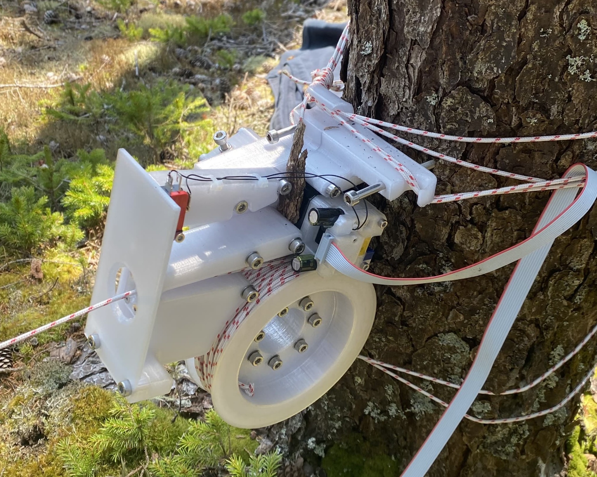
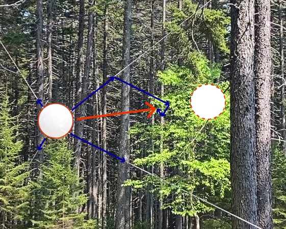
2.8 Discussion
Here I will keep the discussion of these results only to those that are most immediately relevant at the systems layer alone, Chapter 7 explores a broader set of topics that connect through systems design and machine control together.
2.8.1 Key Architectural Limits
There area a few key limits to these systems that I expect are relatively clear by now, but are worth collecting here.
The first set relates to performance and scheduling. Programs in OSAP need to be carefully designed so as not to break the cooperative scheduling routine. So although the systems are designed with the goal of being able to rapidly add new and untested code, doing so can break existing systems. While the MAXL gap enables synchronous operation across high- and low-level systems, the basis spline imposes some additional timing constraints and because the gap is designed against worst-case behaviour it is often larger than it could be. This has to do with scheduling as well because worst case behaviour occurs when the Python runtime is momentarily blocked by either the operating system itself or Python’s own garbage collector.
There are also some key configuration limits; link gateways need to be configured manually within each runtime, and firmwares cannot themselves be modified on the fly, they can only be connected to systems in new ways. The configuration system also requires extensive internal tooling, and even then the types that can be used within PIPES remains somewhat limited. This for example prevented me from including also the model fitting routines in PIPES programs; only the data collection routines are there (I mostly use Python notebooks to fit and analyze data). In the introduction to the thesis I mentioned the goal of connecting entire machine workflows in unified software representations, so these systems come up short in that regard.
One more very important distinction: middlewares enable multicast message passing: one device can write to a topic that may other devices read from. This is in fact a very useful property that PIPES does not currently implement; data transmission in PIPES is strictly point-to-point. To broadcast data to multiple devices we can configure multiple Pipes from the same function, each terminating at a different input. This is not so different in practice but in potentially large systems where very many devices may want to read data from the same source it could be a bottleneck. The network solution to this problem is to use busses as I discussed in Section 2.2.2.2: over busses, a packet that needs to arrive at multiple locations can simply be broadcast over the shared medium — everyone receives a copy. OSAP does not currently support message passing over busses even though it should (2.9.1.1).
2.8.2 Simpler Representations for Composable Systems
One way to articulate the frustrations that I have expressed about machine systems from the state-of-the-art is to say that they are not composable; they are difficult to take apart into pieces and put back together in different arrangements. Machine systems are fragile.
In contrast, music is highly composable: it can be remixed and edited in any number of ways without breaking. This may seem like an absurd comparison, but there are also excellent systems integration tools in music and performance fields that share these properties; MaxMSP, PureData, and OSC are all good examples. All are essentially dataflow systems for music composition and orchestration of not just audio but also lights, cameras, and other ad hoc systems used in performance. Audio also shares timing properties with machine control, in that multiple tracks must be synchronized and computing must be done in a timely manner against a real world constraint.
I thought about these systems often as I developed the architectures here, and I think the key take-away is that simpler representations make composability more likely to emerge.
2.8.2.1 Basis Splines
The cubic basis splines that MAXL uses are the best example of this. In earlier work I used linear segments with additional velocity information to encode motion. Those are perhaps more precise than basis splines because they are direct interpolation, but it is much harder to define how they should be combined. In the basis spline representation, especially where time intervals between each point are uniform, combinations, mixes, etc. are actually very similar to musical tracks. Again StepDance is most similar to MAXL in this regard, and they make explicit mention of tracks and channels of motion data. There are other reasons that basis splines are advantageous at a systems integration level, I discuss those towards the end of this document in Section 7.4.
2.8.2.2 It’s All Tuples to Me
While there is a tendency to want to build abstractions to enable simpler control of hardware, I often found that building firmwares first such that they exposed very simple low-level interfaces provided most of the utility required. It is hard to know how unforeseen applications will want to interface with a module, and abstractions that were meant to simplify can end up adding more complexity than they remove.
Being able to drop these layers (or easily see through them) can be valuable. For example in the Blair Winch project I eschewed all of MAXL but was still able to write motion control by operating the motors’ as simple torque-producing devices directly. I provided a few examples of these simpler systems earlier in the bootstrapping section.
// a global function, defined in the accelerometer
// knuckle's `main.cpp`

auto get_data(void){
  // read, flip, sendy
  auto tup = std::make_tuple(
    data_stamps[data_reading],
    data_accel[data_reading].xData,
    data_accel[data_reading].yData,
    data_accel[data_reading].zData,
    data_gyro[data_reading].xData,
    data_gyro[data_reading].yData,
    data_gyro[data_reading].zData
  );
  data_reading = data_reading ? 0 : 1;
  return tup;
}

// wrapped with PIPES_FUNC to compile a PipesFunctionIFace class.
PIPES_FUNC(get_data, "", "stamp, ax, ay, az, rx, ry, rz");
In the design of PIPES, a breakthrough was to simply use tuples throughout. Serializing, deserializing and naming hierarchically structured data is much more difficult, and if two functions use even slightly different structures reconciling them is nontrivial. Given that embedded systems need to be explicitly typed, this was a tension in the systems design early on. Tuples are much simpler, and the argument mapping and weaving system that I developed in PIPES approximates management of structured data. For example a kinematic component that reads three inputs can be provided with data that is sourced from three separate blocks. This can also be useful in data collection and network management: if we only need a subset of the values produced by a certain function, we can pick them out one-by-one.
2.8.3 Is OSAP an (RT)OS?
I have made some mentions of this question, which pertains mostly to the scheduling problem. Like an operating system, OSAP schedules a set of tasks to run on limited resources. It does so cooperatively, i.e. it cannot stop a task that is already running to run another that has e.g. higher priority. I have mentioned in a few places that this represents a real limit to the systems here overall. Cooperative scheduling is not uncommon, Python and JavaScript both implement “asynchronous” frameworks for concurrent programming; neither truly runs tasks concurrently but simulate doing so with cooperative scheduling. But in realtime systems it is almost a requirement because an uncooperative task can easily cause unsafe operation.
OSAP is also strange in that it primarily schedules packets to handle, not tasks. The proposition there is that in a networked system, packets are a good proxy for subroutines that need to act, and their deadlines are a good proxy for which one should go first. But in PIPES, where we can set functions to run on specific intervals, there is a clear need for preemptive (i.e. uncooperative) scheduling.
There are other benefits to developing OSAP as a “real” operating system, which I will discuss in the future work section (2.9.1).
2.8.4 OSAP and the OSI Model
In the introduction to this chapter I mentioned that the OSI model is only loosely followed, and that it is violated especially in embedded systems where the overhead that network interfaces produce becomes much less acceptable. OSAP makes an attempt to resolve that by clearly separating link, network and transport layers, with PIPES in the application layer. But clearly these systems are interconnected at a deep level: PIPES writes OSAP network routes and extends its discovery layer. I also wrote OSAP with PIPES in mind; to build a compute model that was systems-wide, I developed its runtime to be internally consistent with networks: even though two blocks of software in an OSAP runtime could easily be configured to pass data directly between one another, they do so by writing packets into the runtime’s message stack. In fact most of the value that I propose comes from these three layers (including MAXL) is that they are well aligned with one another. Again the same kind of theme appears; abstractions between components are something of a myth, even or especially at a systems level.
There is an interesting RFC (3439) from The Internet Society [145] that is related. In Section 3 they note:
[…] However, in the data networking context structured layering implies that the functions of each layer are carried out completely before the protocol data unit is passed to the next layer. This means that the optimization of each layer has to be done separately. Such ordering constraints are in conflict with efficient implementation of data manipulation functions. One could accuse the layered model (e.g., TCP/IP and ISO OSI) of causing this conflict. […] For example, layer N may duplicate lower level functionality, e.g., error recovery hop-hop versus end-to-end error recovery. In addition, different layers may need the same information (e.g., timestamp): layer N may need layer N-2 information (e.g., lower layer packet sizes), and the like […]
This is all tightly related to the partitioning problem; to split systems we find that we need to understand them more precisely than existing abstractions reveal.
2.8.5 GCode, Timing and the Partitioning Problem
So, I would like to try to relate all of this to earlier notes in the introduction and background sections. There is a thread in Section 2.1.1 and 2.2.2 on how network performance constrains controller design; programs are limited by compute power, controller distributions are limited by timing constraints, and networks are limited by bandwidth and delay. However, each of these layers is normally separated and so optimally configuring them together is a challenge because representations of the problem change at each layer. This was noted also by [56] in their review of challenges for determinism in cyber-physical systems.
In Section 2.2.3.5 there is a note on how microservice software architectures allow for optimal configurations of distributed software modules in datacenters, and how source routing enables optimal configurations of the networks that connect those modules using software defined networks. Both perform a type of optimization based on policies that declaratively express how configurations should be updated according to dynamic traffic and use.
While they are much simpler and smaller, distributed mechatronic controllers have the same set of constraints. In fact, they have even tighter constraints: the networks we use are typically slower, the programs we write are more sensitive to indeterminism and the embedded devices we use have much less compute power. And they have the additional set of constraints that emerge from the actual hardware that is being controlled; i.e. we need higher bandwidth controllers for systems with smaller physical time constants.
In the state-of-the-art, ensuring that these requirements are met by the system constraints is done by hand. This is one reason why e.g. industrial controllers (2.2.4.2) don’t allow for reconfiguration: their internal control loops and networks are carefully designed such that performance remains deterministic. If Heidenhain allowed machine users to add new software or hardware to existing machines, there would be no way to guarantee that the new composition would not fail. So, this is perhaps another reason why GCode remains where it is; the intermediate layer is useful in this regard because it prevents users from running arbitrary programs on hardware that is designed for performance and safety above all.
On the other hand, we want to bring higher performance, more compute-heavy control methods into these systems. We also want to rapidly assemble systems from modules. This means that we need to articulate the systems integration problem in the same way we would like to articulate machine operation, i.e. as an optimization against constraints that can be discovered rather than defined. The way that I try to move towards that here is to develop inspectable models of operation that span multiple layers of representation. Ideally, each of those could feed information about their constraints and requirements back to systems designers.
Here in the systems chapter I make some progress in that regard (building inspectable models like the SOM), but not much is done about modelling the constraints and requirements. In machine operation I make more progress; in Chapter 4 and Chapter 5 I use machine hardware to assemble component-wise physical models to describe constraints and then optimize over those directly.
So while PIPES, OSAP and MAXL are not ready to robustly solve this problem end-to-end, I think that their architectural deltas from state-of-the-art solutions are worth considering as we take steps towards doing so.
For example the systems object model (2.4.4.1) contains a network map that is overlaid with a software map where data pathways are specified literally in source routes. Function types and transmission intervals are specified directly by PIPES, so it is possible to measure the bandwidths required over each link in the system. MAXL’s explicit timing and “gap” relates those bandwidths to delay. These are requirements, constraints emerge from network performance. The timing analysis in Section 2.7.9 is an example of how networks might be measured, and in Section 2.7.9.4 I relate those measurements to the program’s performance (MAXL). In Section 2.9.1.3, I discuss how network analysis could be improved in OSAP by integrating time synchronization more directly.
This presents an opportunity to build a feedback-based distributed systems design tool that could discover and reflect a distributed control system’s current network loads and limits. That may give designers an interface with which to make intelligent changes either to their networks or software configurations, i.e. modifying their solutions to the partitioning problem against real measurements of constraints.
2.9 Future Work
There are a number of limits to these systems at the moment that I think will be important to manage in the future. The overall goal is ambitious; the hope is to build a set of systems integration tools that almost anyone could interface with to build new mechatronic applications (see Section 8.3). Section 2.8.5 posed the overarching problem: for integration across heterogeneous devices, we need to build tools that allow systems integrators to make sense of the system that they are managing across network, compute, and physical constraints.
I of course have a much longer list of questions and next steps in this regard, but I will try to be concise and high-level here. Organizationally, I will work from the bottom up through OSAP, PIPES and MAXL.
2.9.1 Improvements to OSAP’s Runtime and Structure
I think that the most obvious improvement to make in OSAP overall is for it to graduate as a real RTOS. I mentioned this in Section 2.8.3 and the larger discussion here has circled scheduling, which is at the core of the whole system; we have limited resources but potentially many tasks to complete and messages to send. Scheduling algorithms define how that is managed, and cooperative scheduling cedes authority on the matter to application layer code. Where we endeavor to allow “almost anyone” to put new modules into the framework, this is obviously dangerous.
So, preemption seems like a requirement, see e.g. Section 2.3.2.2.1. Besides actually implementing this (there are well-defined patterns for that), a primary difficult with scheduling is developing a scheme that exposes handles on the problem to system designers. For example in UNIX processes can be given a nice parameter; higher niceness indicates that a process will yield to others more often.
At the moment OSAP is scheduled only based on packet deadlines, which I think is a good proxy for task priority when the system is based on networks. But Pipes Functions that are defined to run at specific intervals need to be included in the same scheme. It is likely that we can simply extend the message stack in OSAP to become a more general purpose task stack that includes these and other tasks. The trouble there is that an interval task that has timed out should perhaps not simply be deleted, and they should neither be run as fast as possible. This means that encoding priorities for both tasks and message passing could become complex.
Treating OSAP more like a real operating system in the Python context could have real benefits as well. The Python interpreter is the main source of indeterminism in these systems, and really it is not a good site for networking. Instead, OSAP could be written in a compiled language for workstation computing and interface to Python blocks via the Port interface, which is already an excellent abstraction for multicore processing. UNIX allows us to dedicate a set of cores to a particular task, OSAP could run there, and Python codes could pass messages to- and from that interstitial layer. This wouldn’t remove the underlying issue that e.g. a motion controller written in Python will sometimes be indeterministic, but it would prevent that code from blocking other network activity.
Addressing multicore operation in embedded devices is also relevant, as more modern chips include two or more CPUs. Because OSAP is based on parallelism and serialization already, this extension should not be exceptionally difficult and the performance benefits could be immense.
2.9.1.1 More (and different) Links
I did reserve some protocol for fieldbusses, but did not implement any in this version of OSAP. They remain highly relevant for distributed control and one ambition in OSAP is to also wrap e.g. CAN or EtherCAT network segments. Overlaying network routes through broadcast layers poses an interesting design challenge; for example consider a packet that is generated in the OS and then travels down a point-to-point link where it is then broadcast over a fieldbus. The route descriptor effectively needs to include a “split over ports” opcode.
There is also the question of remote reconfiguration of links. For example in a system where a control and configuration code first connects to another workstation-scale computer, we should be able to remotely generate a new link in that device to subsequently drill down into hardware attached to it. This may involve extending OSAP’s MVC layers, but it seems more likely that maintaining the separation between custom code and network-specific code is important to avoid cluttering the runtime (which is meant to stay simple). Discovery of available network segment drivers would be one way to manage this.
As I’ve mentioned these links are heterogeneous, we would like to add Bluetooth, WiFi network segments, etc. OSAP’s link gateways can do this, but there are always unforeseen requirements at these layers. There is also the question of more appropriately integrating link-specific capabilities more broadly: WiFi time synchronization (based on simultaneous arrival of wireless packets) can be exceptional, but is specific to the link.
2.9.1.2 More Efficient use of Links
Framing multiple messages into one link frame could be a useful performance boost: if sending and transmitting runtimes need to only encapsulate and decode one packet that contains ten messages the overall processing power and link framing overhead are both reduced. But this again would require more intelligent scheduling; if one message is available to transmit on a link, do you wait for another in some interval before bundling them?
2.9.1.3 About Time
Good time synchronization is clearly valuable for coordinated control and sensing, but it also has value in scheduling and operation of the network itself. The diffusion-based approach that I developed is simple but not as performant as it needs to be to manage extremely high performance systems. It also requires that we tune gains, which should not be the case for heterogeneous systems. Better methods [146] [147] are based on updating estimators for underlying clock skew, rather than controlling skew directly — these approaches look promising. Clock discipline can also be computationally expensive if it is not done carefully, which means that every time a software module has to evaluate the system clock, additional processing overhead is added. On sync itself I will also note that the scheme should be based on “epoch \(ns\),” which is standard in UNIX systems (a 64 bit nanosecond measure of time that has elapsed since January 1st, 1970). Using this as a basis would both improve precision and also allow data captured from even different runtimes to be reconstituted. Aligning against January 1st would require a global reference in each system, that part is probably not required here but would be valuable where available.
Probably the more interesting direction is to make time management more of a core component in the runtime. For example, I described that packet time-to-live is not counted down across a link gateway. But synchronized clocks would enable this, as packet timings could be reconciled across devices. But sync is also stateful; should we want it to be the case that networks don’t work until the synchronization is set up? It may be a worthwhile trade-off to make if this set of architectures is specifically organized for real-time systems.
This could also enable better network and performance feedback. If we can assume that all runtimes have synchronized clocks, writing trace packets that measure network performance becomes straightforward. The same would be true for software profiling, which is another aspect of the scheduling problem. If the real “answer” to the scheduling problem is not better algorithms but better feed-back about its constraints to systems designers, these are key.
2.9.2 Expanding PIPES’ Reach
I mentioned in the introduction that a core tension in this systems design exercise was between simple representations for operation and the capturing of complex software components. But overall, the system ends up lying somewhere in between high- and low-level devices; it was slightly too complex to fit entirely within embedded devices and slightly too simple to completely capture high-level workflows. There are a few steps to take to expand that scope.
2.9.2.1 PIPES Manager in Firmware
Embedded PIPES devices are not reconfigurable in the same way that the Python instances are; we cannot add code modules there on the fly. But doing so would be invaluable. While I have assembled systems that can do these things before, we should bring the same back to PIPES. My master’s thesis includes a version of this [113], which is very similar to the model-view-controller from 2.4.4.1 but including a few more features, namely for instantiating and deleting class instances remotely:
- To load and delete functional blocks, in firmwares, at runtime.
- To register software modules that could be instantiated within a firmware.
- To remotely operate other firmwares and devices, from within firmwares (i.e. outfit the embedded PIPES build with our scripting and systems assembly interface).
The first of these requires some amount of runtime resource management, which brings memory management requirements and can be dangerous in embedded systems without a good RTOS. The second requires (or is difficult to do without) an async API, which is difficult to build in C++, but straightforward in Rust.
2.9.2.2 Improving PIPES Types
Pipes Functions and Classes are also limited in complexity because they can consume and output only plain tuples. This was a key bridge between high and low-level systems (see Section 2.8.2.2), but e.g. most relevant Python codes are written using Numpy. My colleague Quentin Bolsée has noted that the design pattern used within Numpy should be extensible into a system like PIPES, and the typing scheme that we developed together (in Section 2.4.3) includes reservations for this.
Another reservation that Quentin and I share about the current typing system is that the overhead it presents (see Section 2.7.9.2) is too large. One proposal is to hash types rather than encode them directly. That way they could be checked (but not inspected) against a much smaller representation. The other challenge is in PIPES’ argument mapping, which forms a not-insubstantial part of the overhead.
2.9.3 Improvements in Systems Integration Tooling
2.9.3.1 Remote Editing of Source Code
Whereas it is possible to author many of the modules we will want to have available in each of our devices, the current strategy (where they are loaded into devices a priori and then assembled) has two major drawbacks.
- Remote functions become black boxes. Especially because machine design and control mixes nomenclature from multiple domains, it is difficult to ascertain what exactly a functional block actually does from its name and input/output types alone (although types are extremely valuable here). If we could pull source code from these functions as well (or at least, good documentation), much of this confusion could be avoided.
- We can never completely anticipate what functional blocks we will want to build. A great programming point I once heard was something like “my favourite part of dataflow programming systems is the little block I can add that I can write code inside of” — this rings true.
In Python- and JavaScript-based PIPES / OSAP runtimes, this shouldn’t be too much of a challenge, and micropython (a small Python interpreter) may be a good way to implement the same in embedded devices, although that has its own drawbacks. I expect that it is possible to spot-compile functions for a microcontroller and build a kind of partial bootloader to inject new functions on the fly, but this would be a substantial project in itself: it may also be the case that a building a network bootloader handle in OSAP is enough, and where we want to add new blocks we simply recompile the device’s entire firmware, reload it, and reset it. In any case, the value in being able to completely describe a distributed system in this manner is sure to be of major importance if we go towards trying to build robust, safe, and verifiable systems in an architecture like this.
2.9.3.2 Developing a Visual Graph Interface
It is clear that the systems deployed in this thesis are (1) always distributed and (2) sometimes messy. Structurally, they are all graphs, but I do not have a tool to visualize them as such. I would like to build a tool to do so.
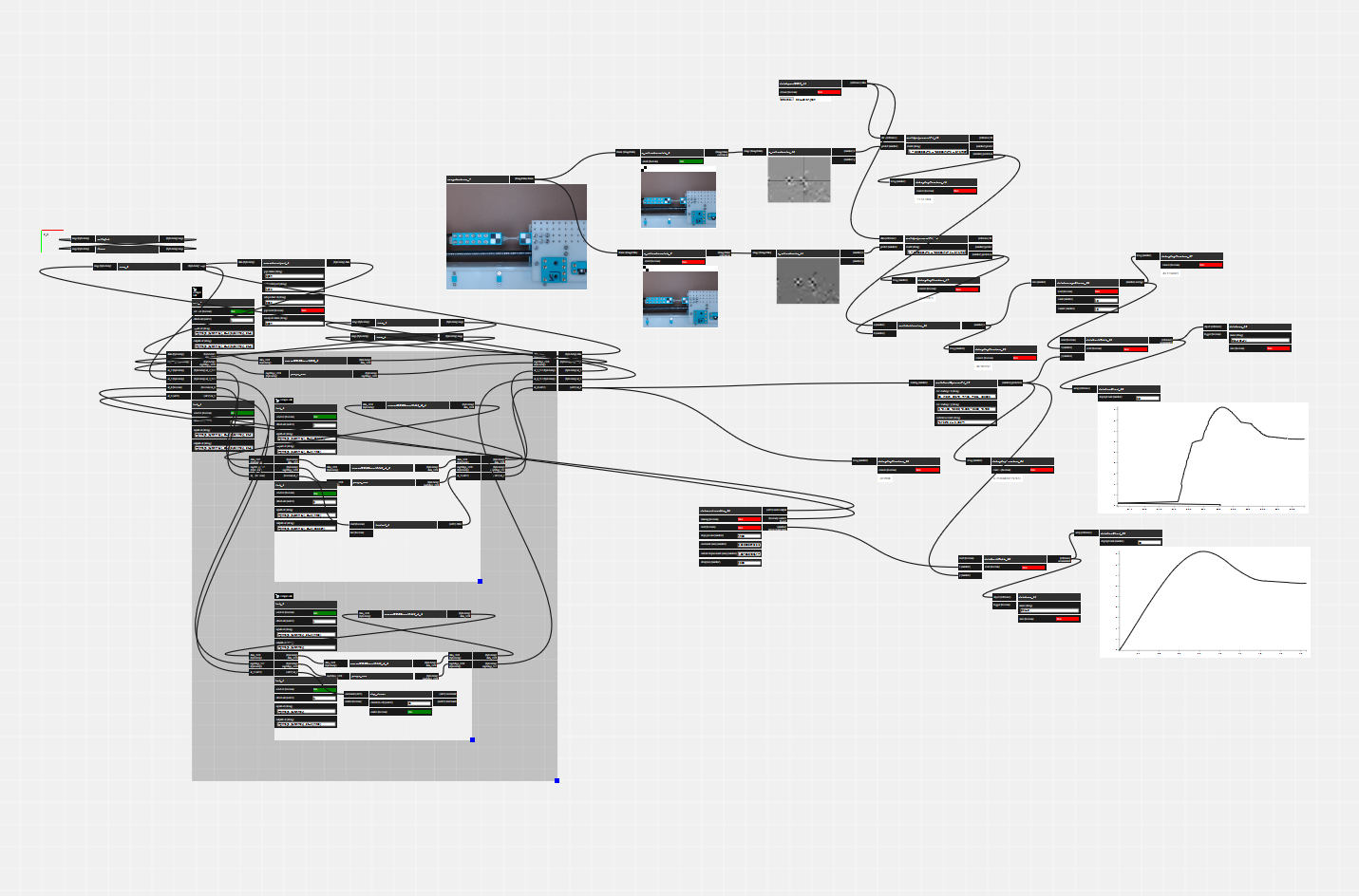
A graph visualizer and editor would let systems developers quickly debug which hardware modules are connected, inspect their APIs, and build low-level data streams between devices. I have built a similar system in the past, but made the mistake of over burdening the graph representation: programs there had to be described entirely as graph entities. In an updated version, I would like to be able to interchangeably use scripting and graphs.
2.9.4 Redistributing MAXL
I designed MAXL with the intention of using it to more easily reconfigure distributed motion controllers. In the implementations in this thesis, most of the MAXL blocks run inside an OSAP Python runtime, but the programming model is extensible across runtimes; the CoreXY block (or any other) could be instantiated in firmware if it were authored there in C++.
However, doing this with flexible reconfiguration within embedded devices (not just of embedded devices) would require the work that I described in Section 2.9.2.1 to be complete. The advantage gained from doing so is maybe clear by now: network and determinism based constraints (the partitioning problem!) mean that it is valuable to be able to relocate some parts of a controller into “the edges” where latency is lower and determinism is higher.
I’ve already mentioned Ilan Moyer’s StepDance [95]; its characteristics are representative of what I am imagining here: responsive, realtime control using composable mathematic blocks. StepDance uses firmware-level block configurations step-and-direction to encode motion (sometimes using a specialized encoding to transmit more than one channel of step-and-direction over the same wire), whereas MAXL uses basis splines and time synchronization. That introduces the gap (Section 2.5.2), which introduces at least some delay between trajectory generation and execution. The size of that gap is based on network latency, and can be set accordingly; Section 2.9.1.3 discusses how measurements made by OSAP can be used to estimate how minimal this gap can be — but latencies and determinism of software components also figures. This is why profiling tools for networks and for software blocks in OSAP and PIPES are also important next steps.
This is especially true for responsive control interfaces and realtime control loops. Despite all the feedback via models that is shown in this thesis, I do not mix very much realtime feedback into control flows, besides at very low levels. But we can imagine using MAXL and PIPES blocks as a basis for mixing and reconfiguring consistently timed control loops, e.g. driving load cell data into a PID pressure controller that drives a torque signal into the extruder motor (see Section 5.12.3.1). Upstream planners could transmit tracking signals to that controller.
2.9.4.1 Using Local Look-Ahead
For a final note, queuing motion as a function of time also opens up the possibility of using smaller look-ahead controller within each device. As we drive performance of our motor drivers in the future (and continue to develop better models of these systems, and more embedded compute performance), using small model-predictive controllers for look-ahead may become more prevalent and common (at the moment most practical controllers are simple PID loops). These require that each device has a future window of control commands to inspect, and time-encoded basis splines will be a useful representation in these cases.
In even simpler scenarios, some devices have known (and constant) lag times between actuation and output: for example an electromagnet or solenoid driven at the same voltage will always have the same delay (between when voltage is applied and when the target current is reached). Devices with fixed lag can simply inspect their target trajectory that many milliseconds in the future, and begin actuation ahead of time in order to delete lags.
2.9.4.2 Expansion of MAXL Flow Types
In the earlier MAXL paper [110], I developed a more complete set of “track types” that could encode motion or e.g. events, sensor trigger timings, etc. These are harder to synchronously model alongside basis splines (what does it mean to multiply two even channels with uneven timings together?) but maybe the solution to that composability problem is actually simple. There are many potential use-cases for those types of tracks, and I think that their re-integration is worth exploring.
2.9.4.3 In-Firmware Safety Backstops
Finally, but perhaps a critical piece of work, is the notion of pushing safety critical control into lower level devices. In a number of places I’ve mentioned that one trade-off with model / optimization-based controllers is that they are less deterministic and inspectable by nature. I worked to make the velocity planner that I develop in Chapter 4 more inspectable than other end-to-end approaches, but because it models sometimes messy physics it remains unclear to me if it can be made completely deterministic (see Section 4.8.3). Other advanced controllers (like reinforcement-learning methods) are surely not deterministic. Networks are also never \(100\%\) reliable, especially here where we are proposing to add “almost any” link layer technology.
But we still want to deploy these systems in practice because they provide invaluable performance and capability improvements. At the moment I do have simple backstops in MAXL’s spline interpolator; if one point is missing, but the two adjacent points are present it is easy to add the missing point between the others. More robust versions of this type of approach could be developed, for example running a per-device energy minimization policy where packets are missed.
References
When multiple configurations at multiple layers in the system are set up manually and cannot be easily checked, errors can easily emerge if any of those configurations disagree with one another due to human errors or misunderstandings.↩︎
Layer interfaces and abstractions add computing and memory overhead.↩︎
For example, a difference in network architecture from one machine to another is OK when those two machines don’t need to be interconnected as part of a larger system as is the case for the internet, where connection to the network itself is the main activity. In fact, there is some industrial pressure to maintain architectural differences in networking technologies because these can form the basis of intellectual property “moats.”↩︎
In a DDoS (Distributed Denial-of-Service) attack, networks are flooded with malicious packets and as routers try to manage this surge in traffic, they collapse.↩︎
The word scheduling in computer science broadly refers to this task: the problem first really became relevant when the first operating systems were developed (to share one CPU across many programs). It is NP-Hard.↩︎
For example, good solutions to the scheduling problem can help to improve CPU performance substantially, so there is significant work on the topic.↩︎
In the introduction I wrote a section on how machines are poorly represented (1.3.2), Object Oriented Hardware is the clearest way to begin solving this problem.↩︎
Who appears in this thesis’ acknowledgements, and who I have been lucky enough to spend time and share research notes with during especially the latter half of my time at MIT.↩︎
Who is one of my co-advisors on this thesis, and whose guidance as I have developed these tools has been invaluable.↩︎
How we might build simpler and more stateless networks and machine controllers has been a long-standing question posed by my advisor Neil Gershenfeld.↩︎
See more on source routing in Section 2.2.2.2.↩︎
I discuss
modsin more detail alongside other tools like it in Section 2.2.4.7.↩︎Python is a popular scripting-based programming language that has been widely adopted by scientists, engineers, backend developers etc.↩︎
It is common for GCode interpreters to be configured for different tasks using a firmware sourcecode file called i.e.
config.hwhere system settings are changed. To update settings, we modify this file and recompile the firmware. More modern firmwares allow these configurations to be read and written remotely, normally through an auxiliary interface but sometimes through custom GCodes.↩︎Networks tend to collapse when they approach their maximum utilization. The typical pattern is that increasing congestion starts to cause packet loss, after which transport layer algorithms begin queuing extra messages (retransmits), further increasing congestion. Once everyone starts doing this, links are quickly saturated and performance bottlenecks. Much work has gone into developing transport algorithms that intelligently avoid and recover from these scenarios, i.e. TCP New Vegas (which uses packet delay, rather than packet loss, as a flow-control signal).↩︎
I was once debugging a packet loss issue for nearly half of a day before I realized that the cable (containing UART over RS485) was lying on top of a switching power supply that was emitting noise in around the same frequency of the link’s bitrate. I moved the cable and the performance was restored. Wireless links are the same: too many cellphones in a room and your bluetooth headphones or WiFi performance will degrade.↩︎
For an example from this thesis, the motor controllers (Section 4.4) are using all of their available 200MHz to servo the motors around. If we tried to stick the motion controller in there as well (and more motors), things would explode. This is additionally true for compute in general: datacenters and supercomputers rely on networks to expand compute volume beyond what is available on a single die.↩︎
“Clock Discipline:” a term of art meaning the strategy with which we actually skew our local clock against the network clock.↩︎
A clear explanation of middleware from the Distributed Systems textbook [59]: “To assist in the development of distributed applications, distributed systems are often organized to have a separate layer of software that is logically placed on top of the respective operating systems of the computers that are part of the system […] In a sense, middleware is the same to a distributed system as what an operating system is to a computer: a manager of resources offering its applications to efficiently share and deploy those resources across a network.”↩︎
Message formats in ROS are not strictly standardized, they are more akin to naming conventions, for example
/tffor robot transforms,/scanfor laser scans,/joint_statesfor joint positions. Software packages are set up by default to look in these pseudo-standard locations, but can be configured otherwise.↩︎For an example of an MVC interaction: you (the user) request to trade \(\$1000 \text{USD}\) of virtual money in your bank’s ledger for cash at an ATM. The ATM sends a request to the controller in the bank’s backend software. It checks if you have this many virtual dollars in the ledger and if you do (and you have authenticated yourself), it subtracts those from the ledger (updating its model) and returns a new view to the ATM: your updated bank balance, and then a subsequent request to the ATM’s controller to dispense the dollar bills. The ATM dispenses the cash and then updates its internal model of its cash stores.↩︎
High speed stepper pulse timing is an important performance metric for these systems, as I discuss in some more detail in Section 7.4.2.↩︎
Programmers will normally think of “ports” as the interfaces they use to communicate into a network, so when we are talking about OSAP’s internals, this can become confused with “links,” which are what point out of OSAP into network segments.↩︎
This seemed like a lot when the project started, but it should likely be expanded with an additional byte for 15 bit port addresses (32 768 ports).↩︎
Trace packets can be used in some networks to measure performance. As they move through networks, they append timestamps into their datagrams and information about the location of the timestamp — see Section 2.9.1.3.↩︎
Memory allocation is one of the main functions that operating systems perform and doing it poorly can lead to severe and difficult to trace bugs.↩︎
This may too aggressively over simplify the scheduling problem, see Section 2.9.1 for a note on improvements.↩︎
For simplicity and robustness this is based on the runtime’s own accounting of time, not the system synchronized time.↩︎
PI is proportional-integral control: to generate a control output, one control gain (for P) is multiplied by the error, and another (the I) is multiplied by an integrated error signal.↩︎
In embedded systems Pipes are allocated from a fixed-size pool that is instantiated in the runtime’s memory (its size can be configured at compile time), a common design pattern and similar in nature to the one that I described for OSAP’s packet access scheme in Section 2.3.1.4.↩︎
This represents a current limit in the PIPES system. In the work in this thesis it did not become problematic, but a more principled design may include provisions to configure functions with improved flow control rules at the PIPES level, e.g. not consuming new data from inputs until all Pipes are cleared — or configuring these rules on a per-Pipe basis.↩︎
For example in MAXL blocks where it is important that we generate only one new output on each tick of the timer, but we have woven inputs to one of these blocks, the
on_all_freshinput mode will hold operation until each input has received new data from upstream blocks. The CoreXY and BedLevel blocks in Figure 2.10 use this input mode. MAXL’s operating logic is described in Section 2.5.1.↩︎I discuss how we might add this capability to embedded systems in Section 2.9.2.1.↩︎
NPM, the Node Package Manage and PIP, the Package Installer for Python, are registries of software modules that can be used by programmers to rapidly build new applications.↩︎
Is OSAP an RTOS? See 2.8.3 for discussion on whether it really qualifies for this label.↩︎
The load cell’s comparator function is a good example of something that could be added on-the-fly to an embedded device if lower-level program reconfiguration were possible, which I explore in Section 2.9.2.1. It is a small software-defined module (so it does not need to be device-specific) that reduces bandwidth requirements for some applications: rather than sending data from a sensor all the time, send it only when a signal reaches a certain (configurable) threshold. It is also something that not every device developer may think needs to be included in their hardware; I only developed it once I need to perform this bed levelling procedure, so I took a loop through the firmware update and proxy collection cycle that I explained in Section 2.7.2.↩︎