The End of GCode
Machine Architectures for Feedback Systems Assembly
PhD Thesis Proposal
Jake Robert Read
MIT Center for Bits and Atoms
Neil Gershenfeld
Director, Center for Bits and Atoms
Massachusetts Institute of Technology
Director, Center for Bits and Atoms
Massachusetts Institute of Technology
Nadya Peek
Associate Professor, Human Centered Design and Engineering
University of Washington
Associate Professor, Human Centered Design and Engineering
University of Washington
Jon Seppala
Director, nSoft Consortium
National Institute of Standards and Technology
Director, nSoft Consortium
National Institute of Standards and Technology
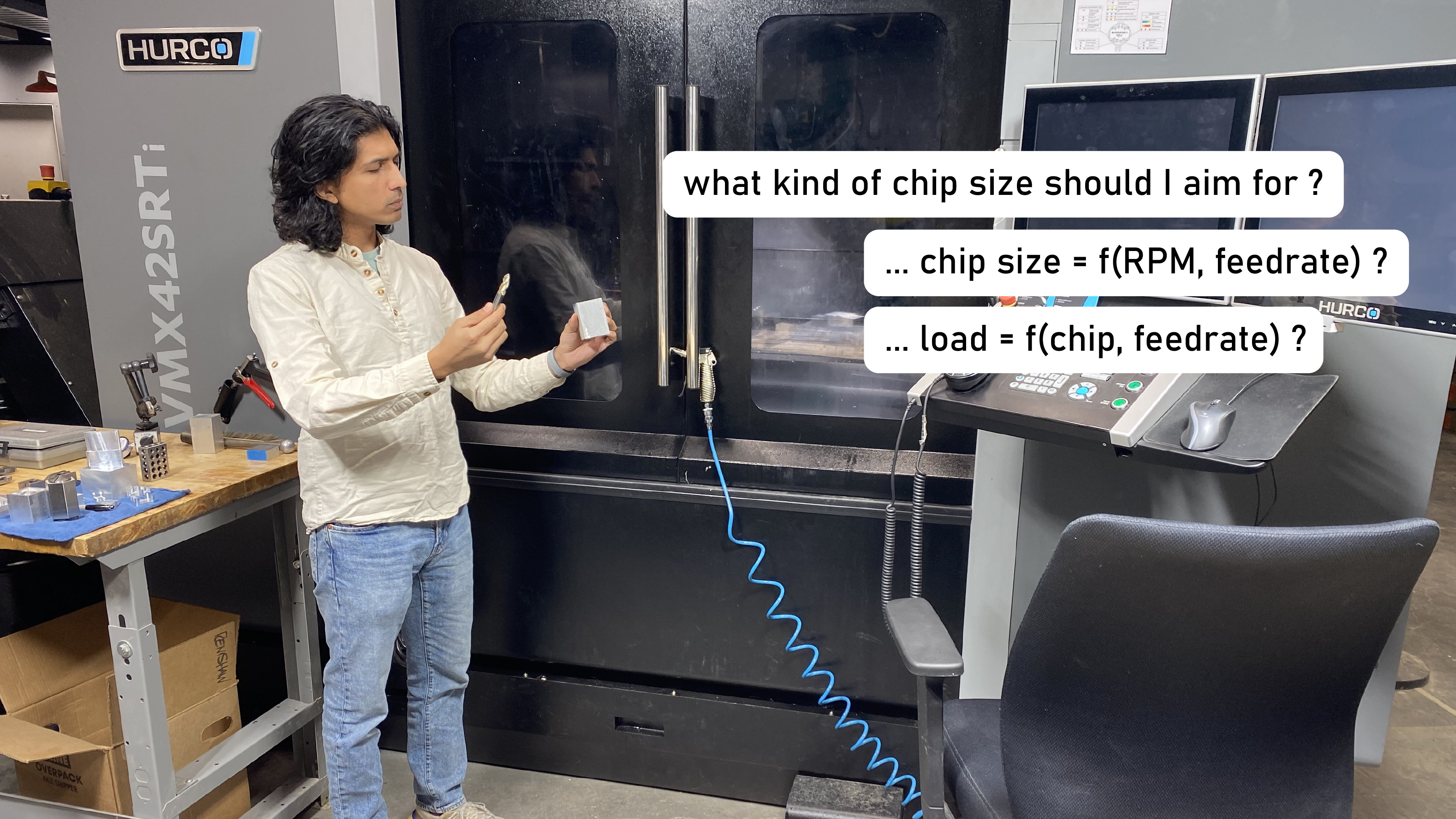
How can we make it easier to use and understand machines?
How can we make it easier to develop and improve machines?
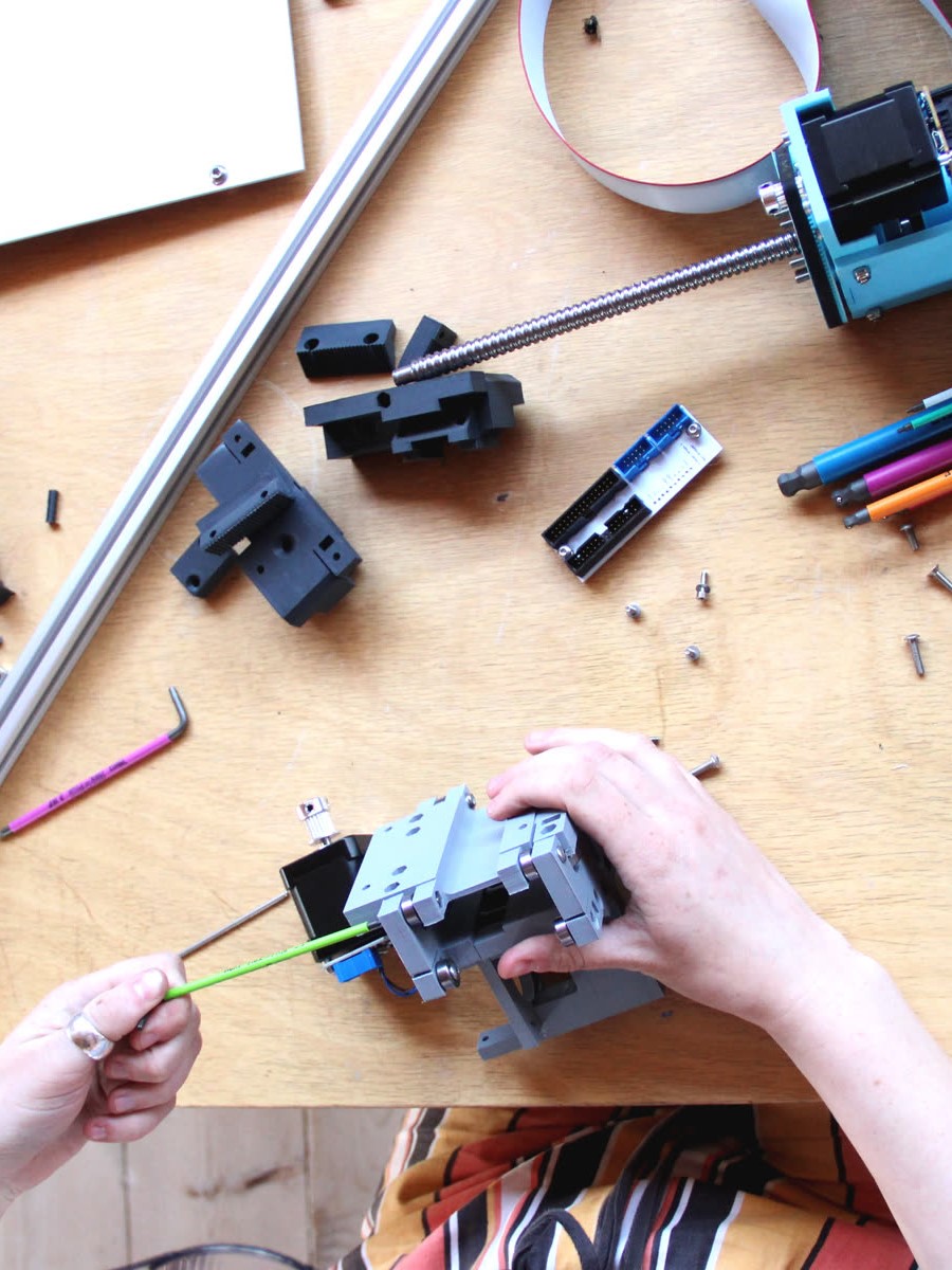
Peek, Nadya, et al. "Making at a distance: teaching hands-on courses during the pandemic."
Extended Abstracts of the 2021 CHI Conference on Human Factors in Computing Systems. 2021.
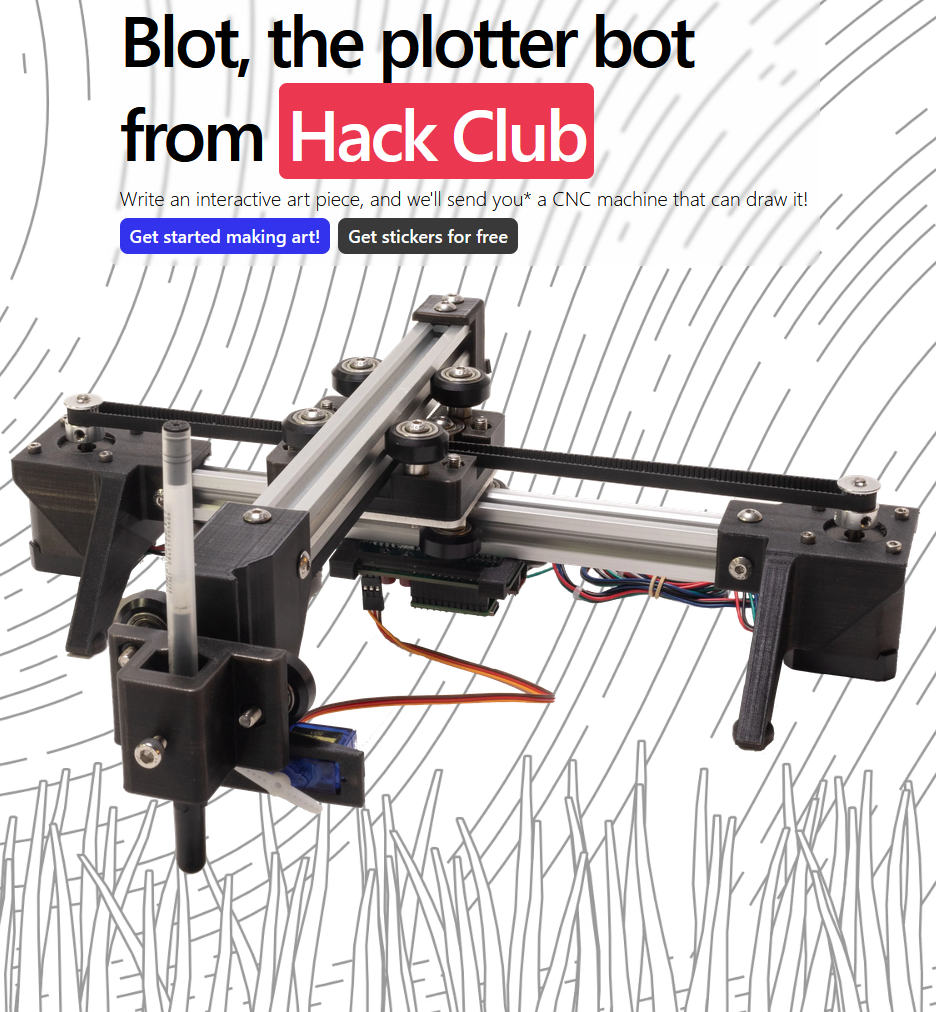
Hack Club and Leo McElroy
https://blot.hackclub.com/
https://blot.hackclub.com/
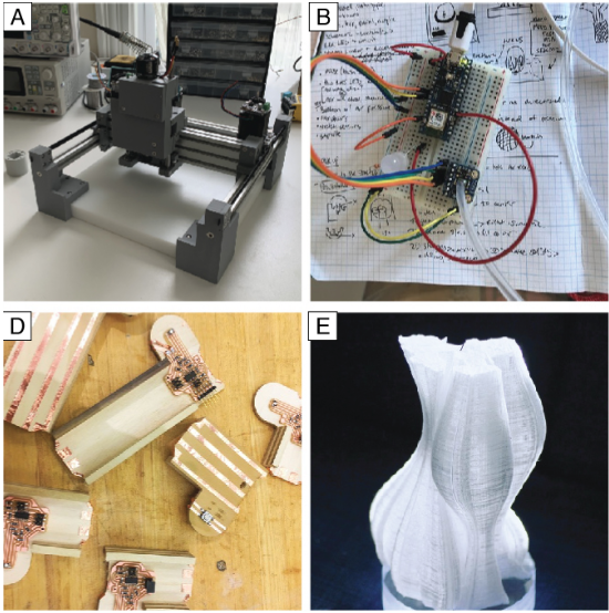
Vasquez, Joshua, et al. "Jubilee Demo: An Extensible Machine for Multi-Tool Fabrication."
Extended Abstracts of the 2020 CHI Conference on Human Factors in Computing Systems. 2020.
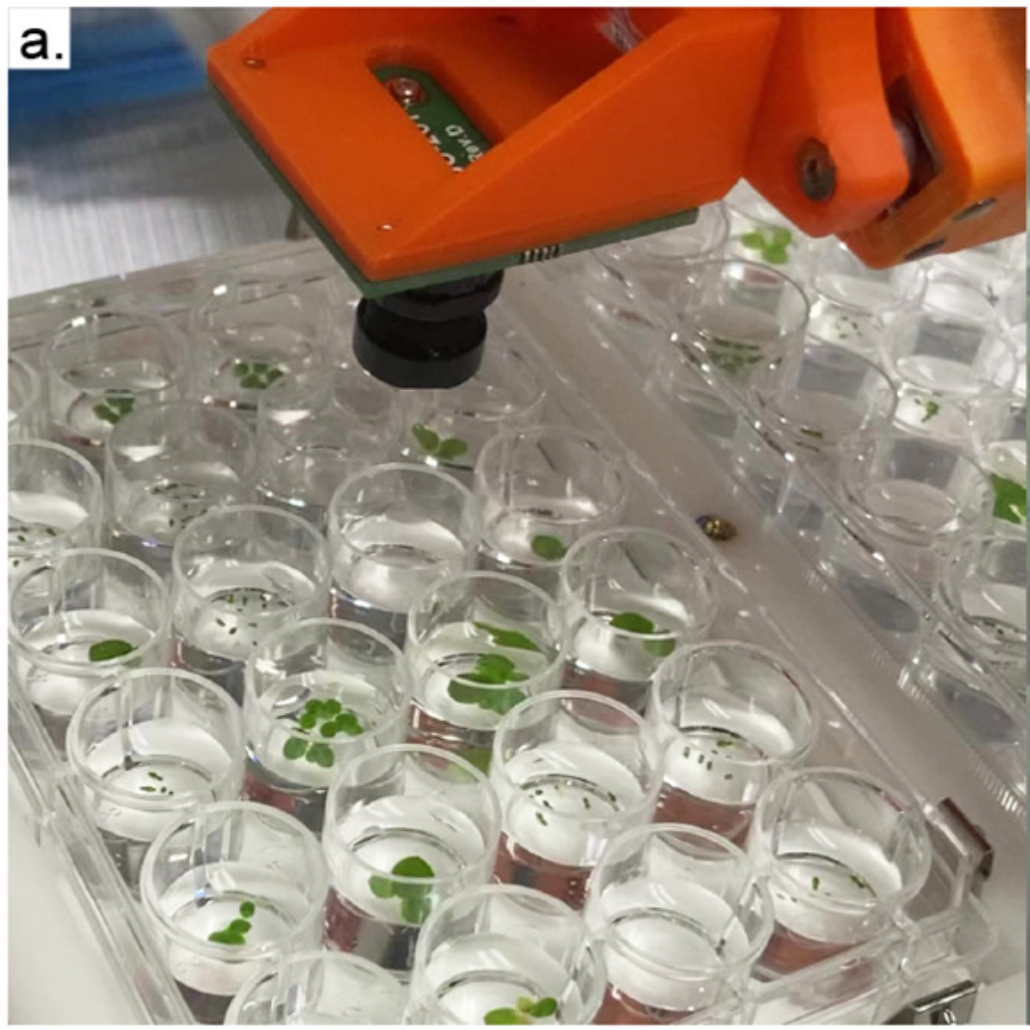
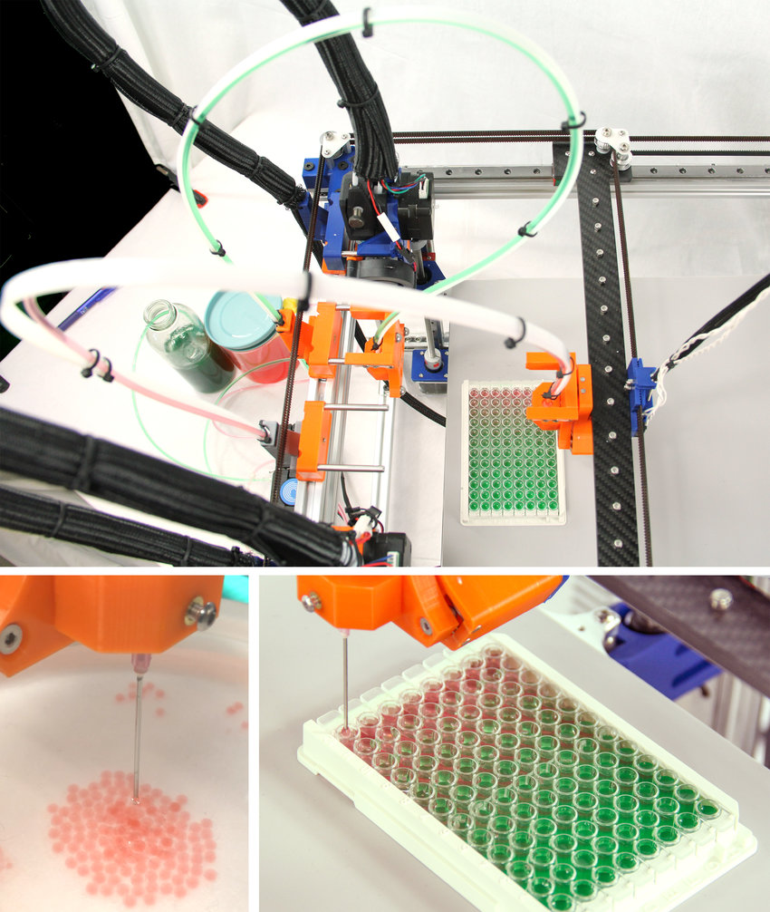
Subbaraman, Blair, et al. "The Duckbot: A system for automated imaging and manipulation of
duckweed." Plos one 19.1 (2024): e0296717.
Strieth-Kalthoff, Felix, et al. "Delocalized, asynchronous, closed-loop discovery of organic
laser emitters." Science 384.6697 (2024): eadk9227.
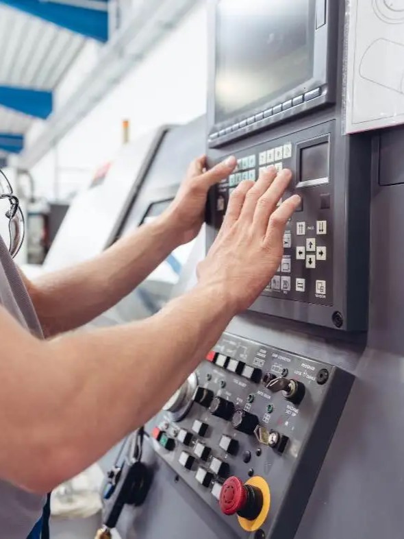
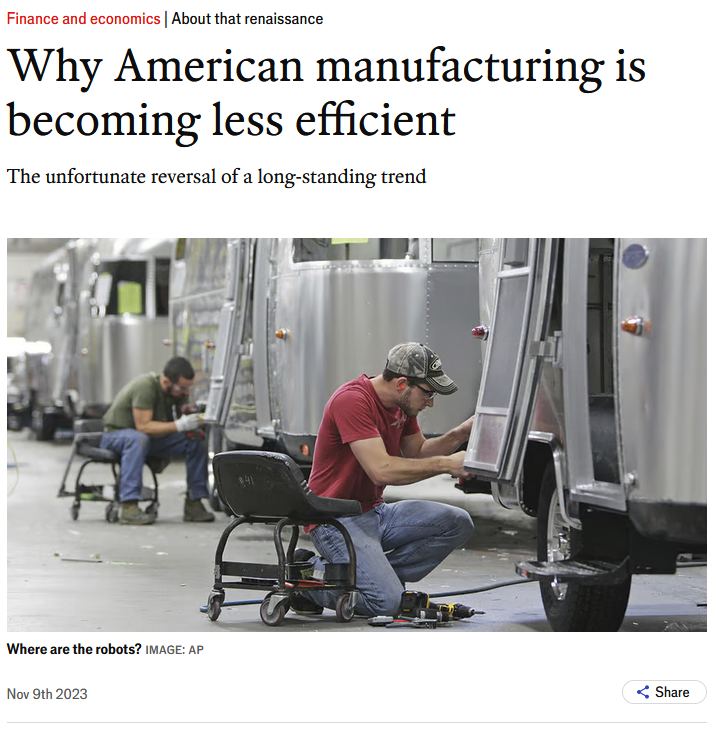
From The
Economist
Nor can we improve those jobs' productivity; we aren't developing new automation rapidly
enough.
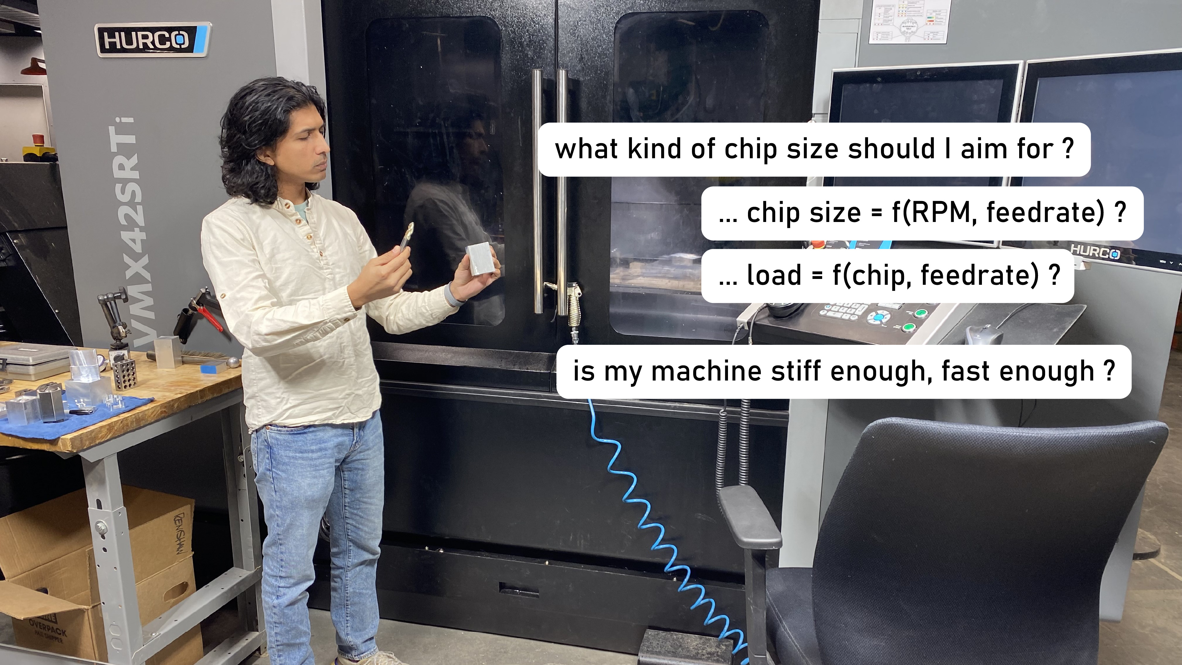
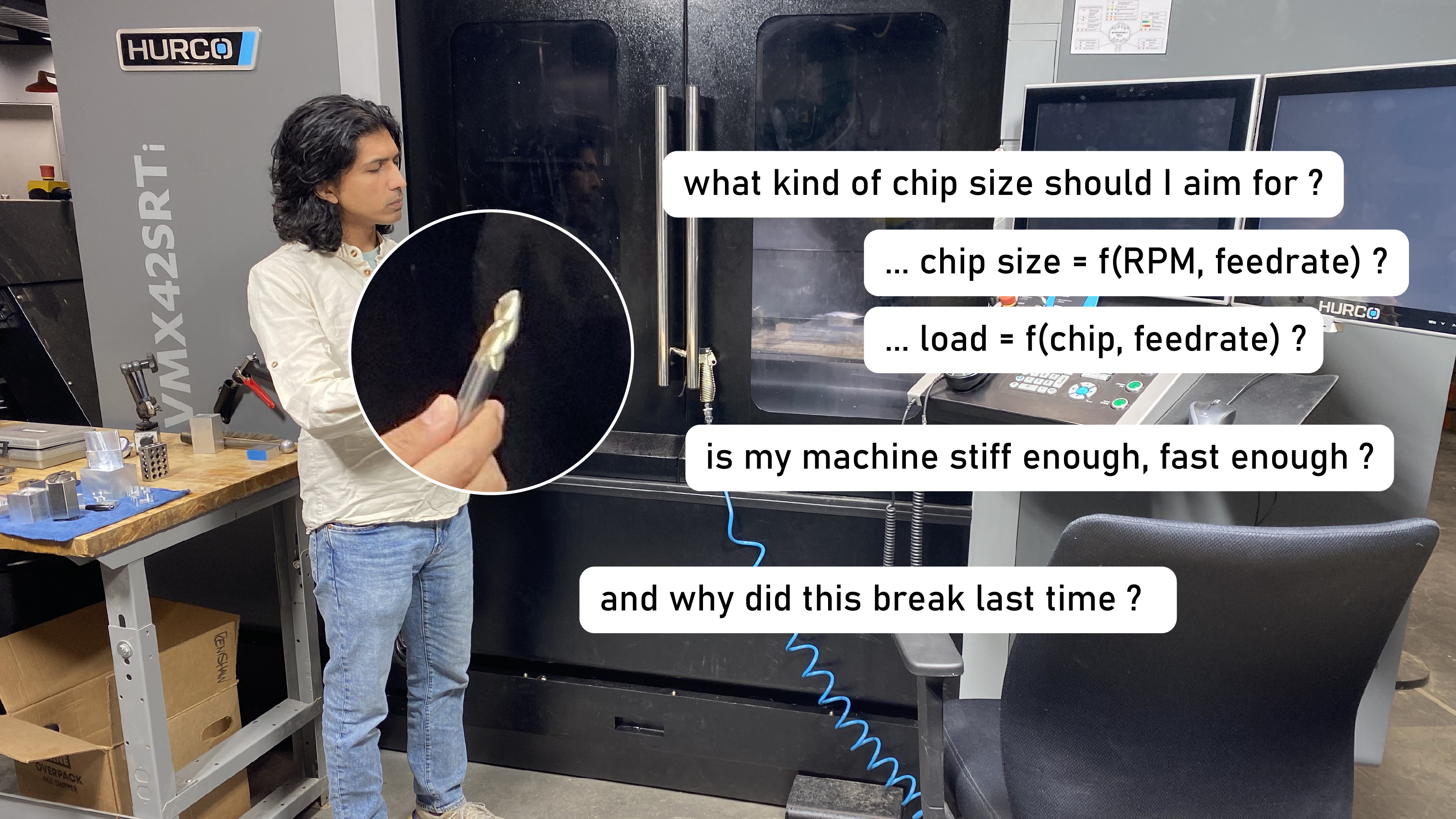
Proposing to replace...
Best-guess, iterative parameter tuning.
With...
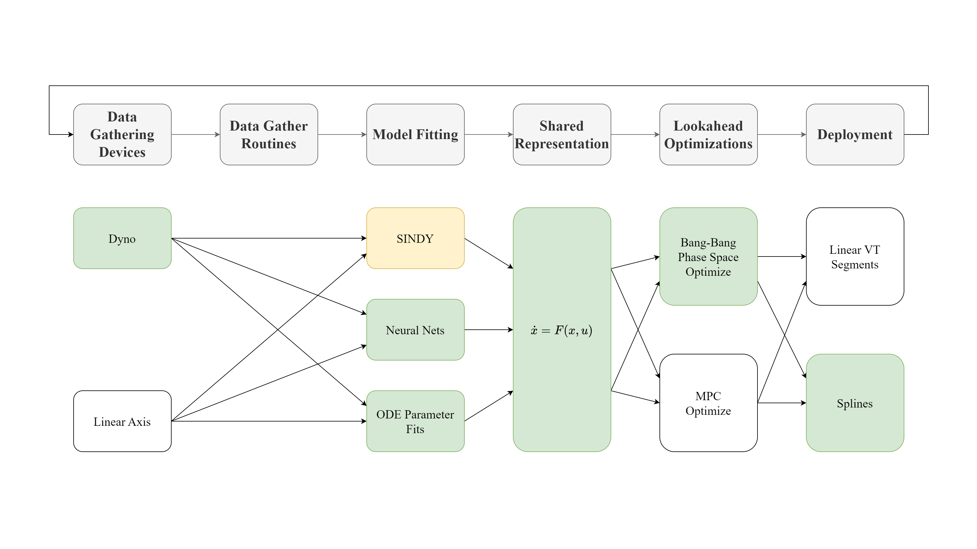
Models of machine physics generated with in-situ data.
Guarantee that we don't exceed physical limits.
Improve performance by operating close to those limits.
A more intuitive tool for users to understand their equipment.
With...
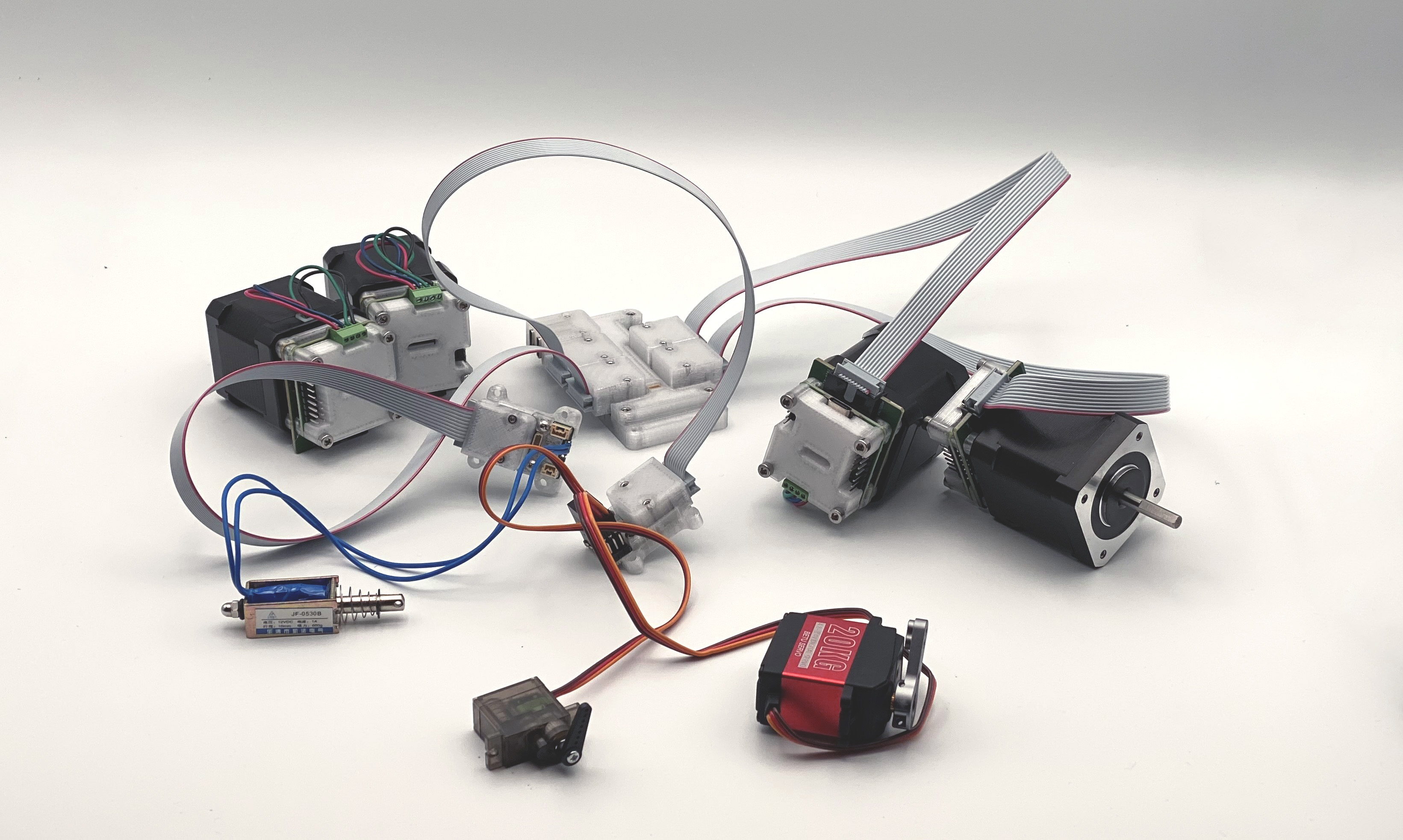
Modular distributed controllers based on feedback.
Span multiple layers of configuration and control.
Generate as much data as they consume.
Interface to digital twins.
G21 ; use millimeters
G28 ; run the homing routine
G92 X110 Y120 Z30 ; set current position to (110, 120, 30)
G0 X10 Y10 Z10 F6000 ; "rapid" in *units per minute*
M3 S5000 ; turn the spindle on, at 5000 RPM
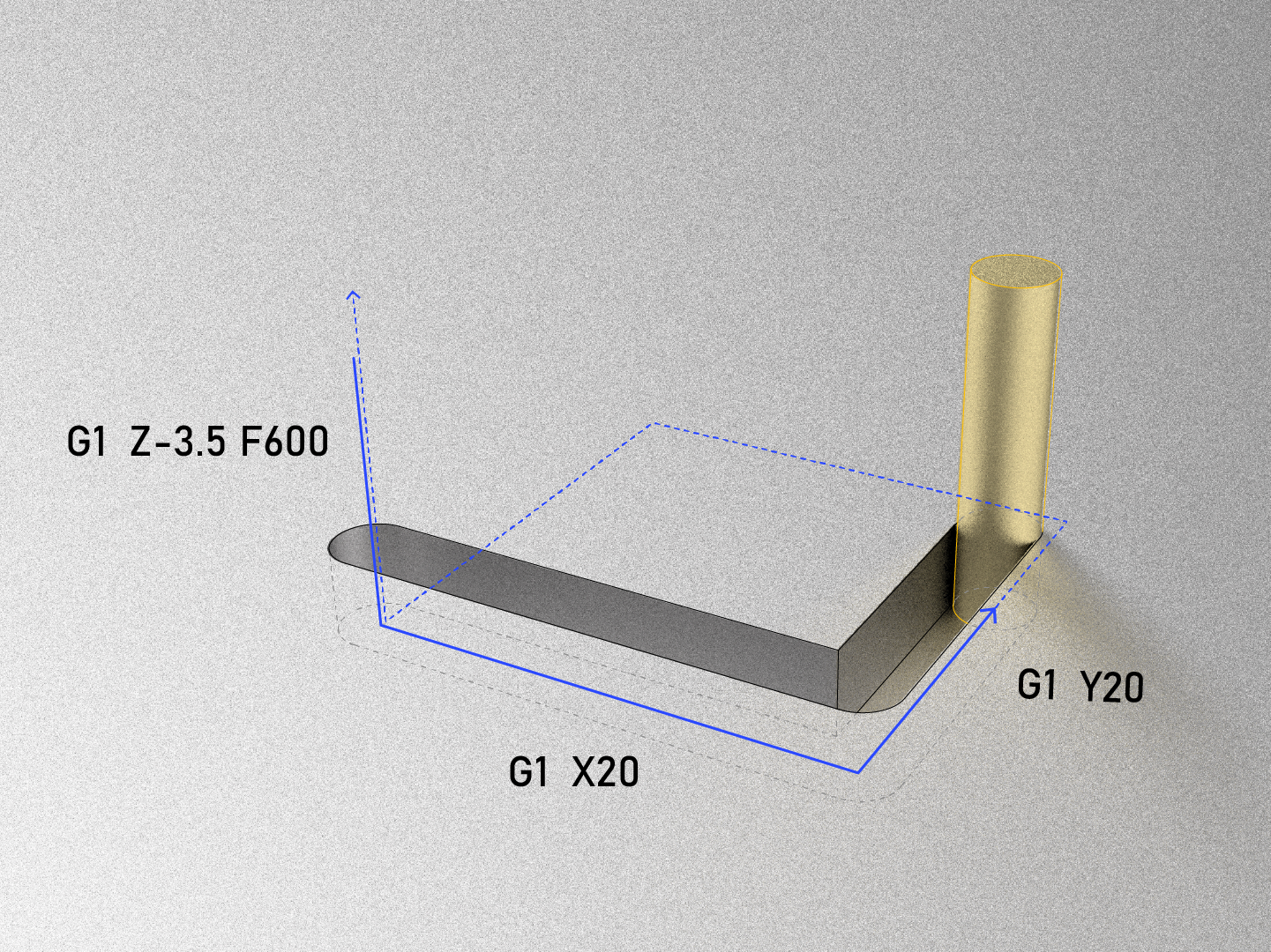
G1 Z-3.5 F600 ; plunge from (10, 10, 10) to (10, 10, -3.5)
G1 X20 ; draw a square, go to the right,
G1 Y20 ; go backwards 10mm
G1 X10 ; go to the left 10mm
G1 Y10 ; go forwards 10mm
G1 Z10 ; go up to Z10, exiting the material
M5 ; stop the spindle
G0 X110 Y120 Z30 ; return to the position after homing (at 6000)
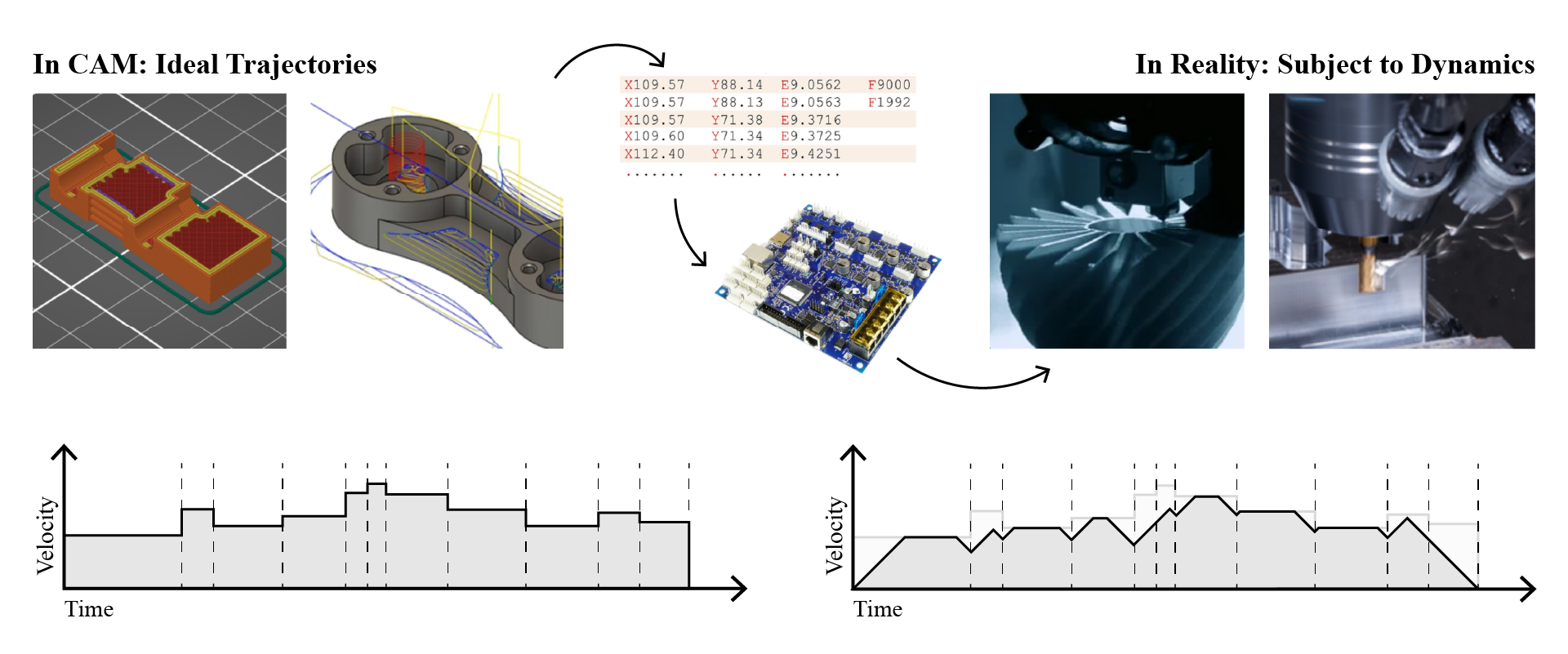
A simple GCode program, for a milling machine.
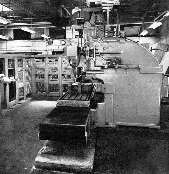
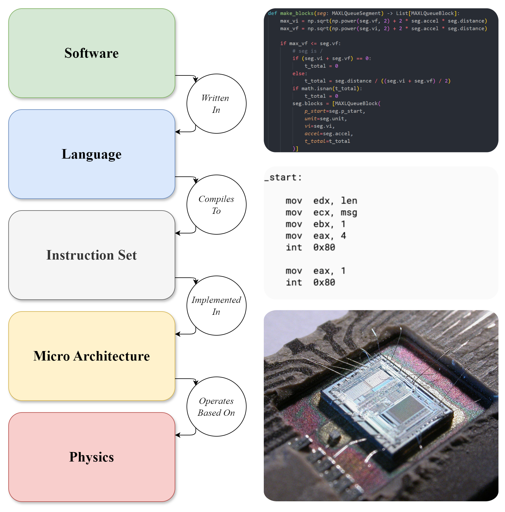
GCode was invented alongside the first CNC machine, in a milieu of computer scientists who were
developing top-down, feed-forward design patterns for system abstraction.
Noble, David. Forces of production: A social history of industrial automation. Routledge, 2017.

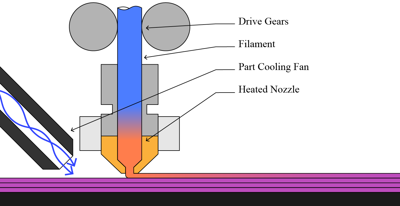
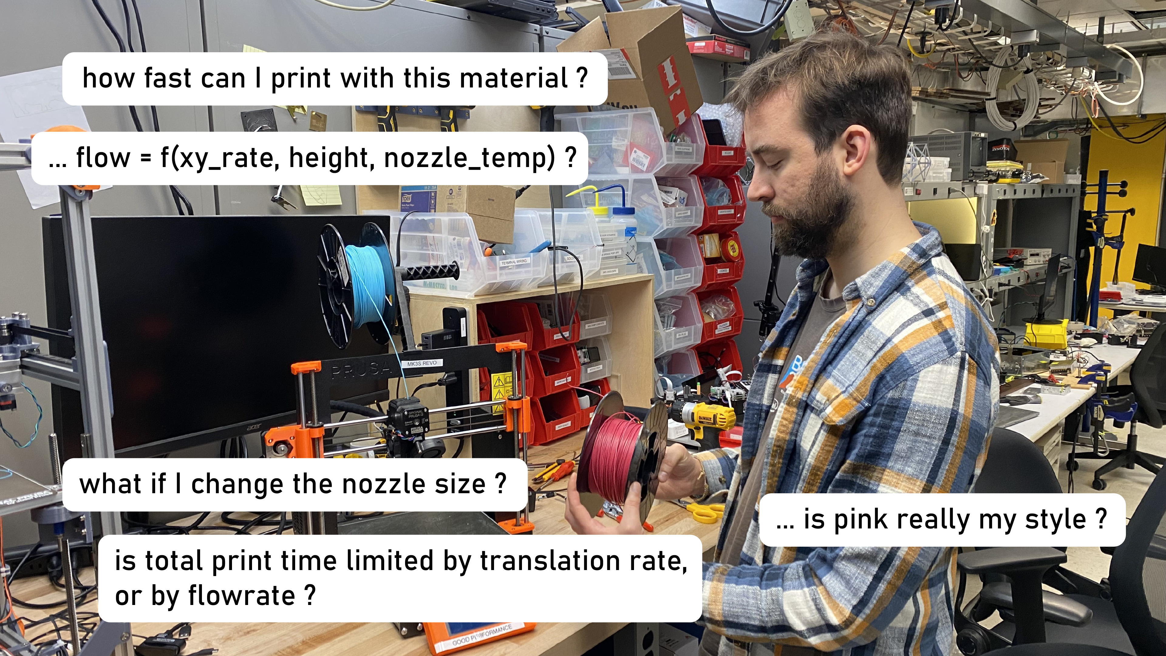
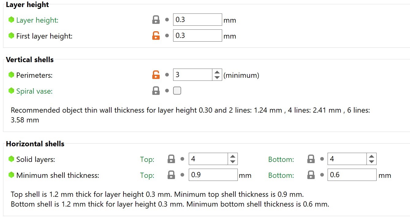
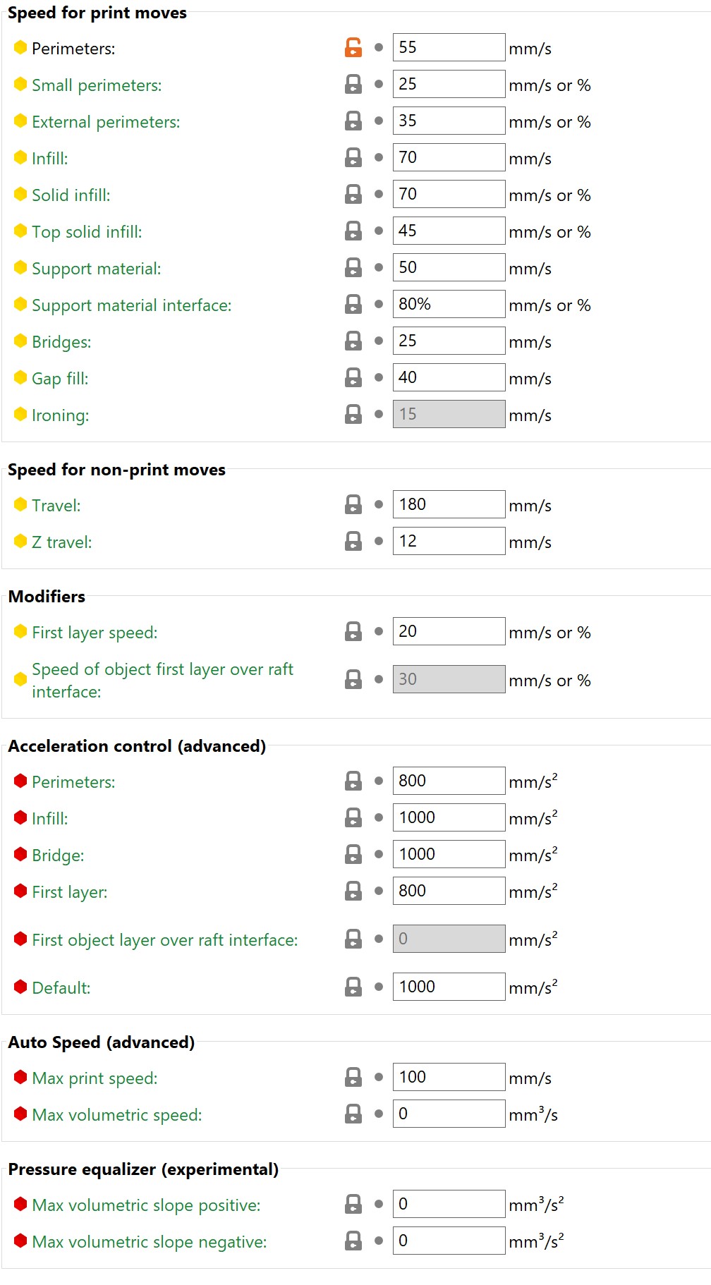
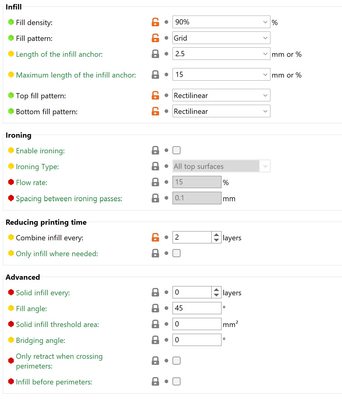
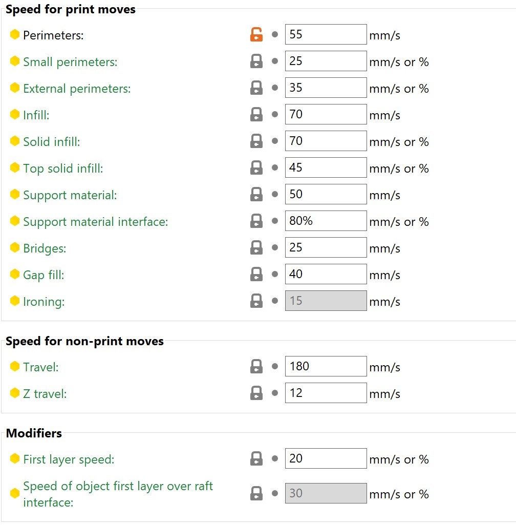
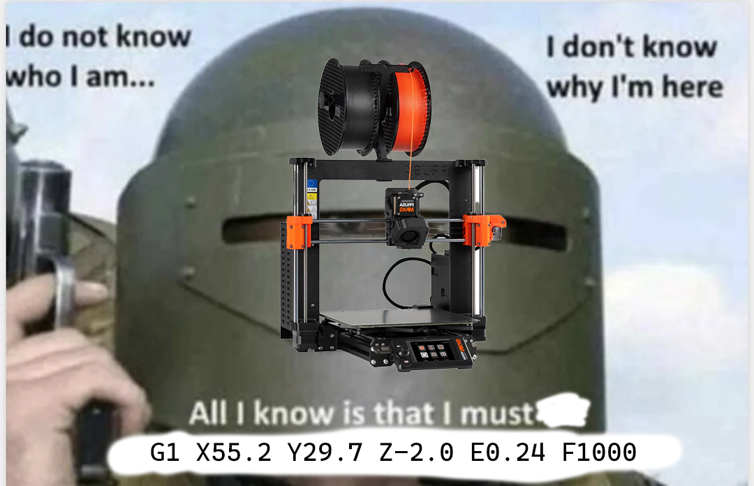
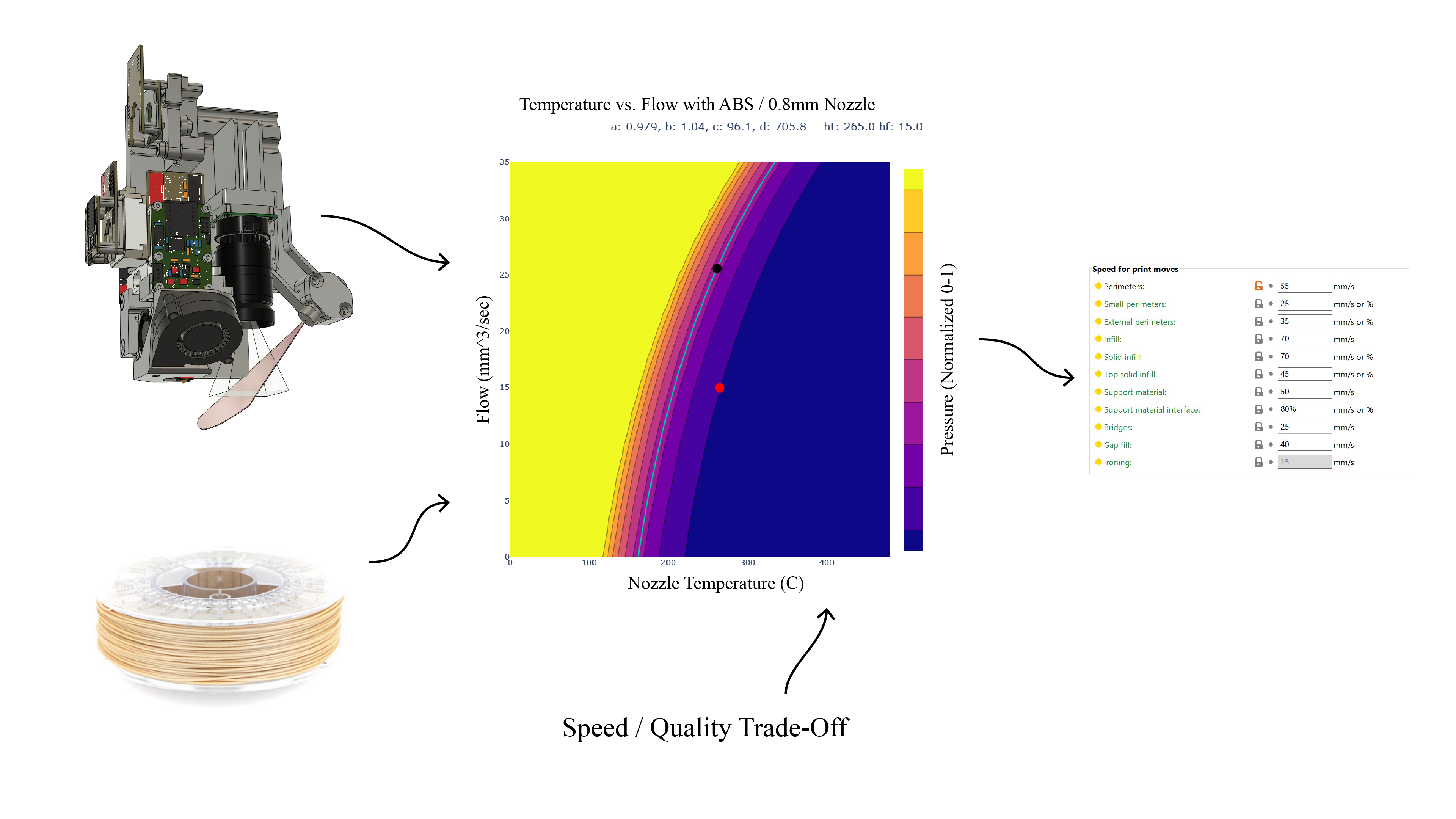
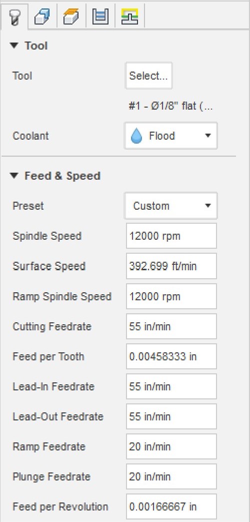
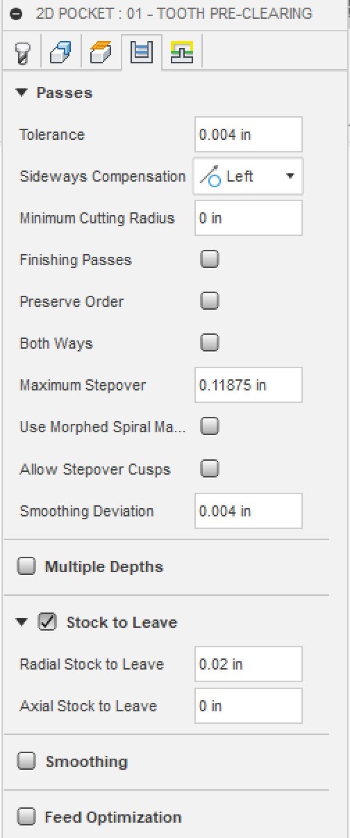
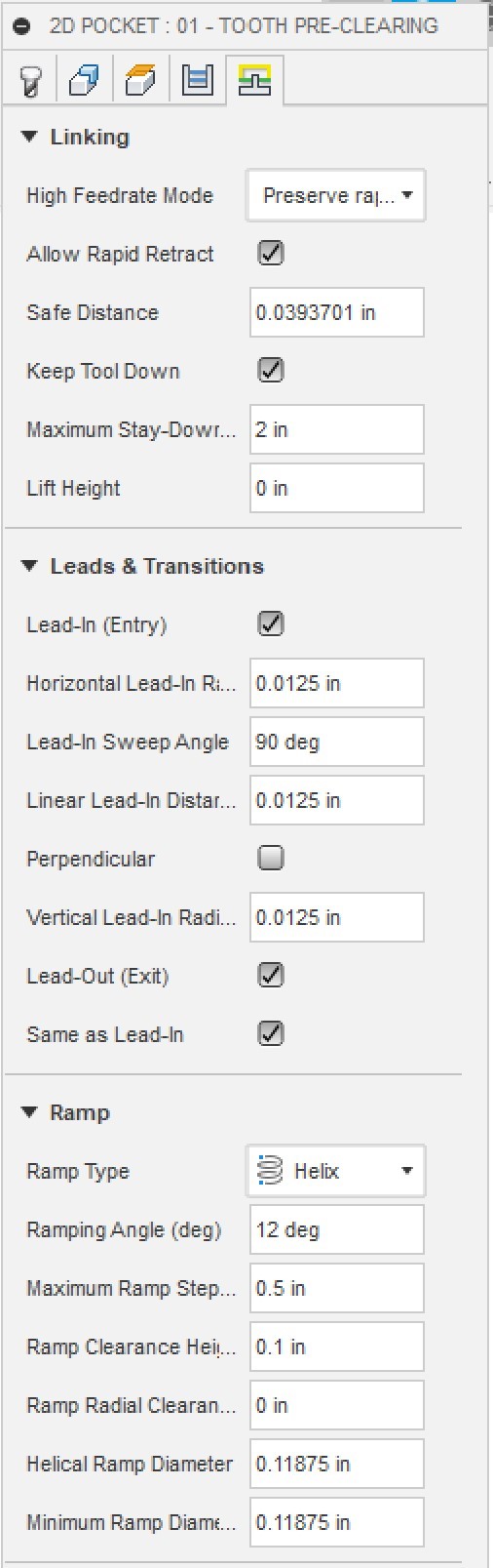
3D Printing Parameters as shown to users in PrusaSlicer
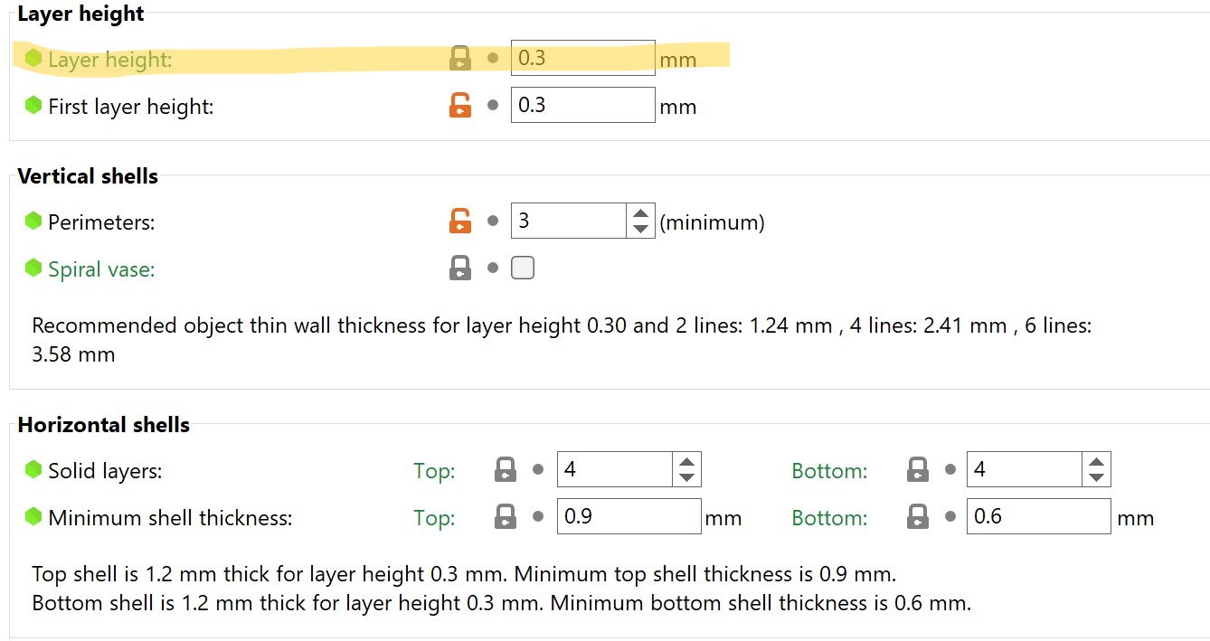
3D Printing Parameters as shown to users in PrusaSlicer
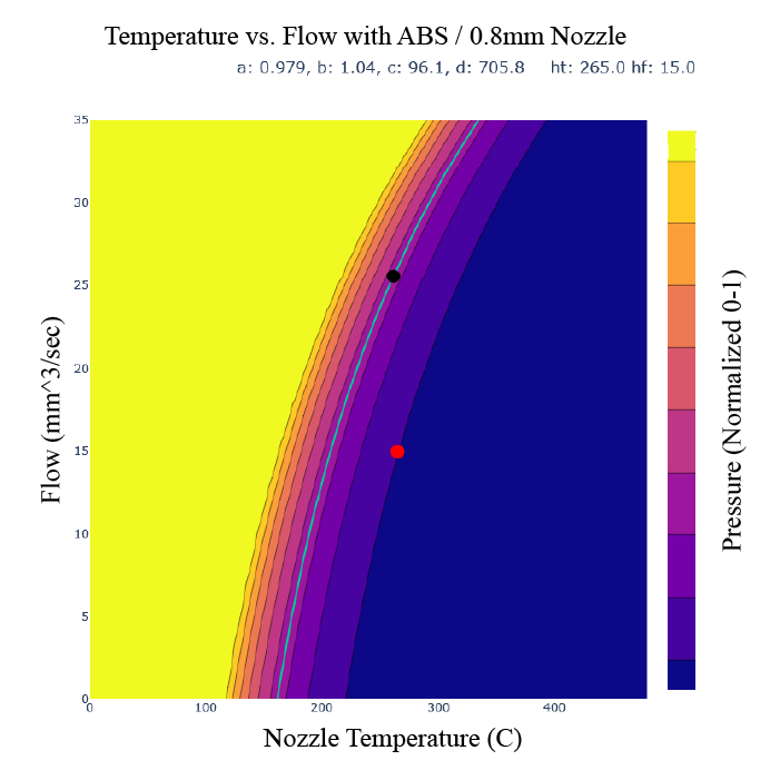
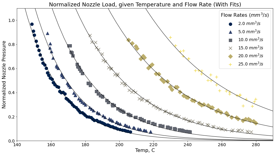
Coogan, Timothy J, and David O Kazmer. 2019. “In-Line Rheological Monitoring of Fused Deposition Modeling.” Journal of Rheology 63 (1): 141-55.
Kazmer, David O., Austin R. Colon, Amy M. Peterson, and Sun Kyoung Kim. 2021. “Concurrent Characterization of Compressibility and Viscosity in Extrusion-Based Additive Manufacturing of Acrylonitrile Butadiene Styrene with Fault Diagnoses.” Additive Manufacturing 46 (October): 102106. https://doi.org/10.1016/j.addma.2021.102106.
Wu, Pinyi. 2024. “Modeling and Feedforward Deposition Control in Fused Filament Fabrication.”
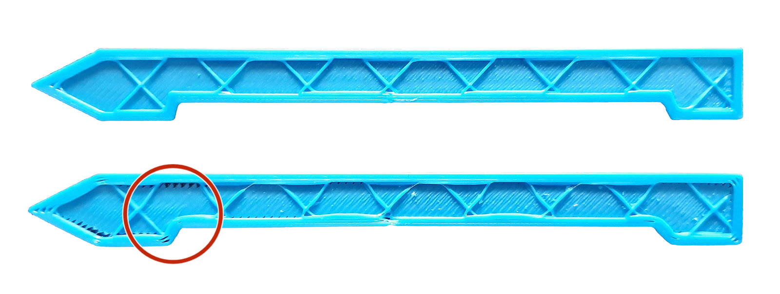
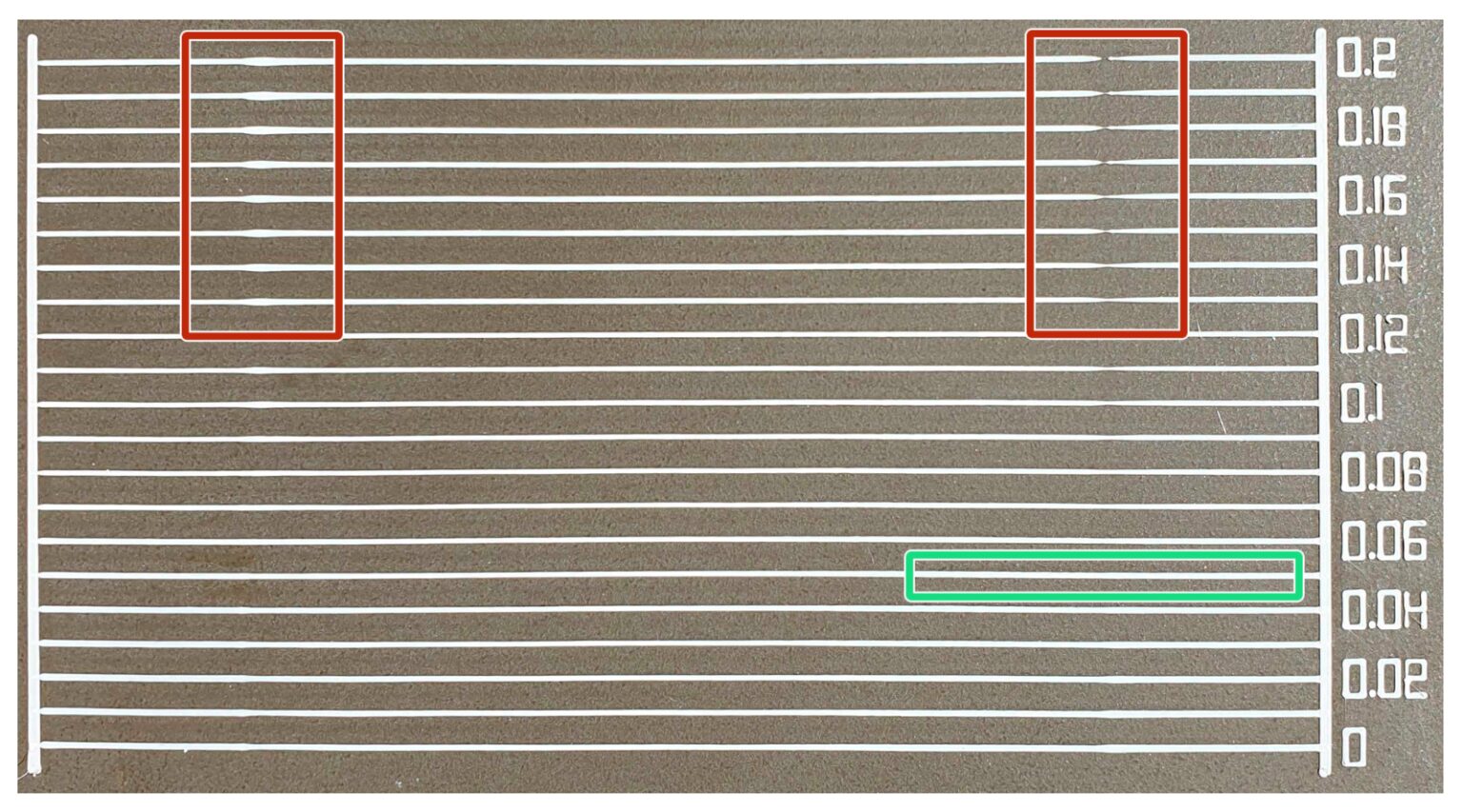
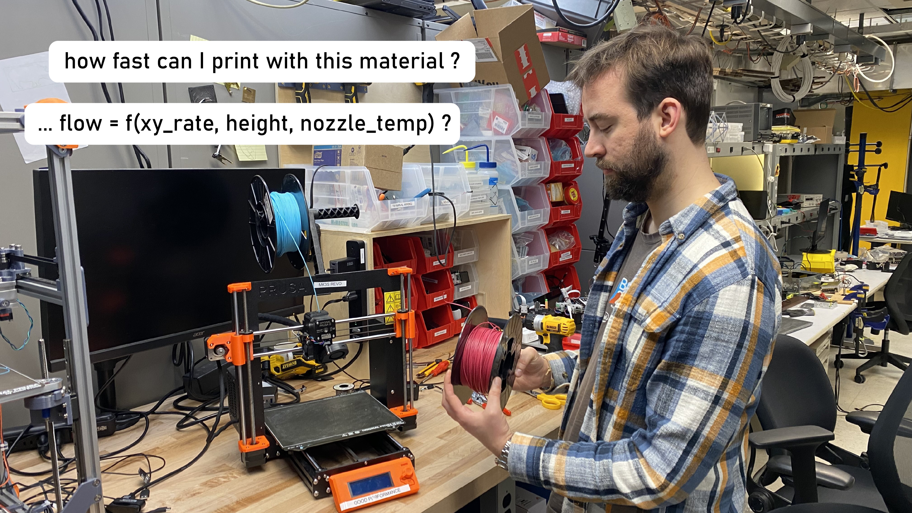
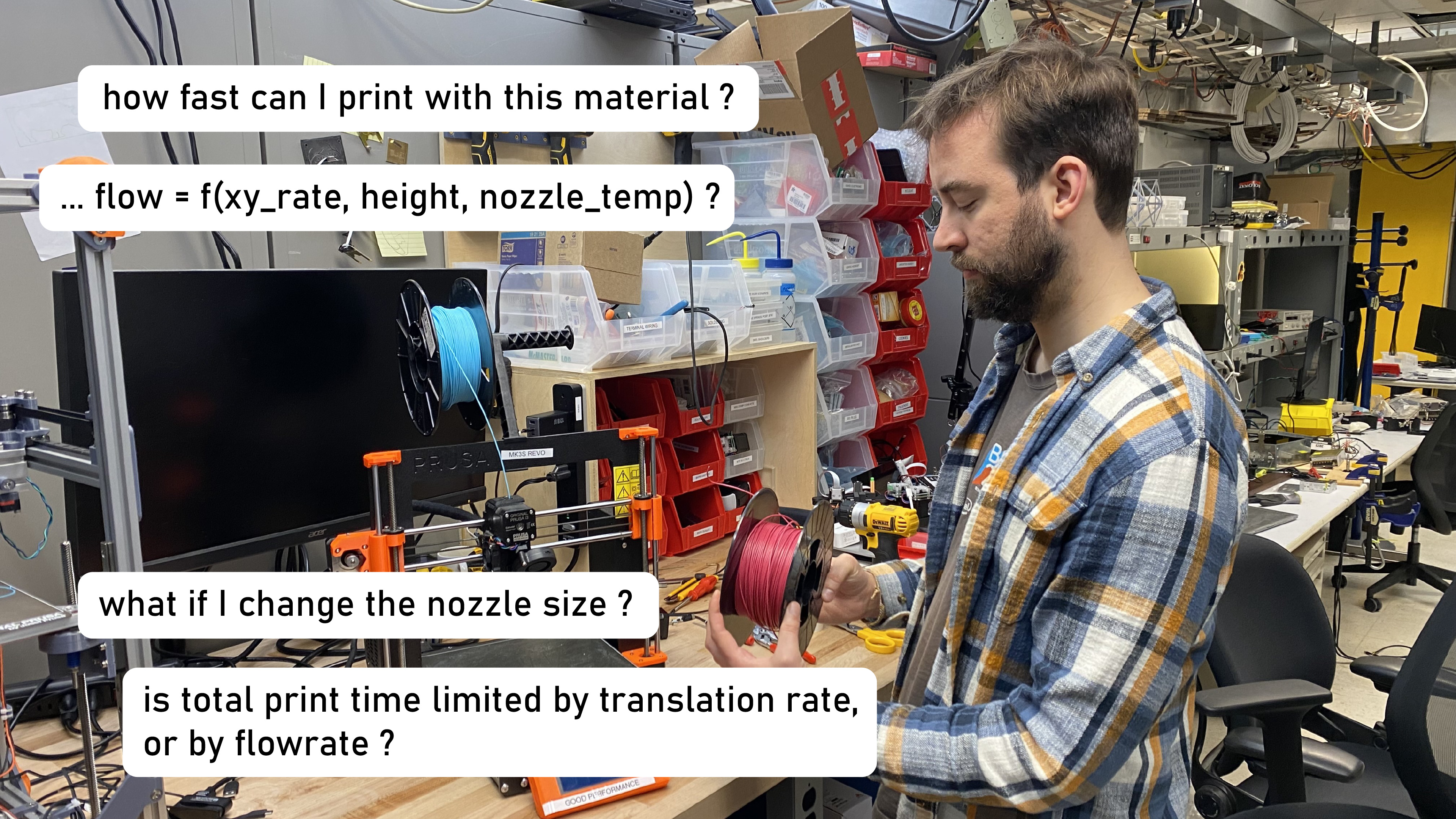
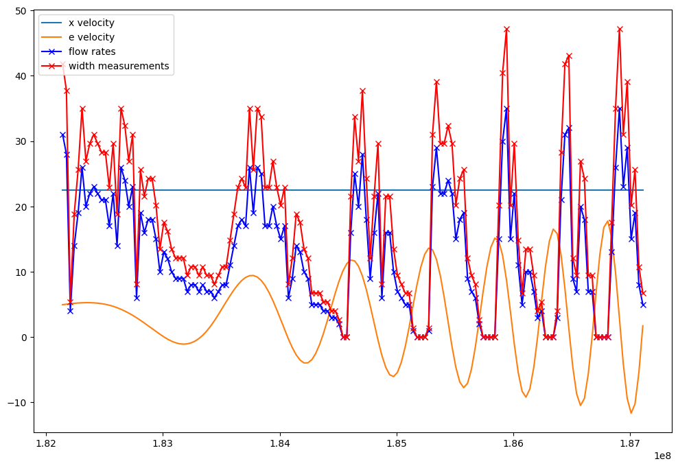
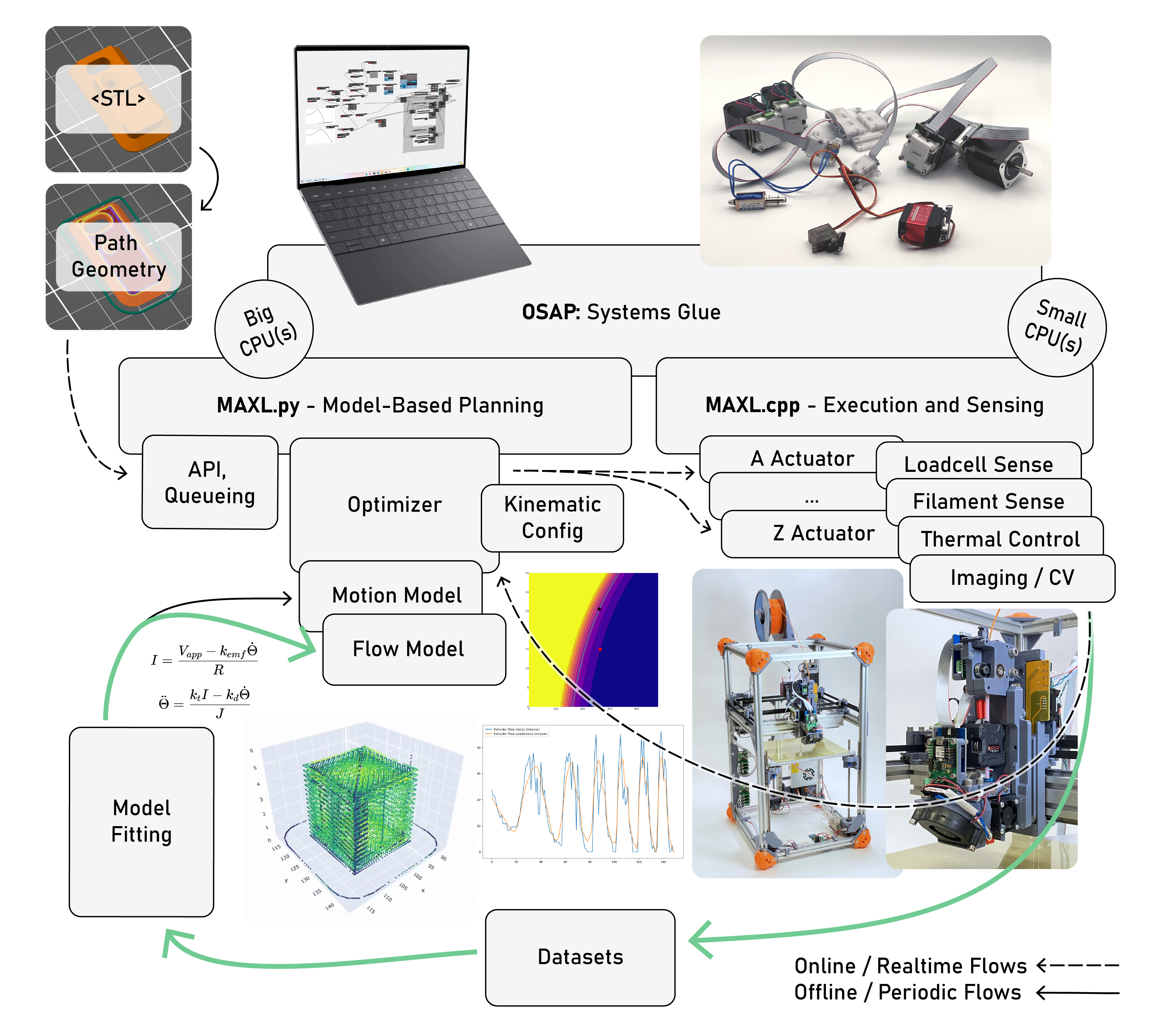
Using track width w/ lateral speed and layer
height to measure flow. W/ Yuval Mamana
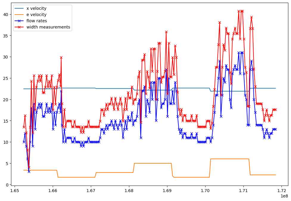
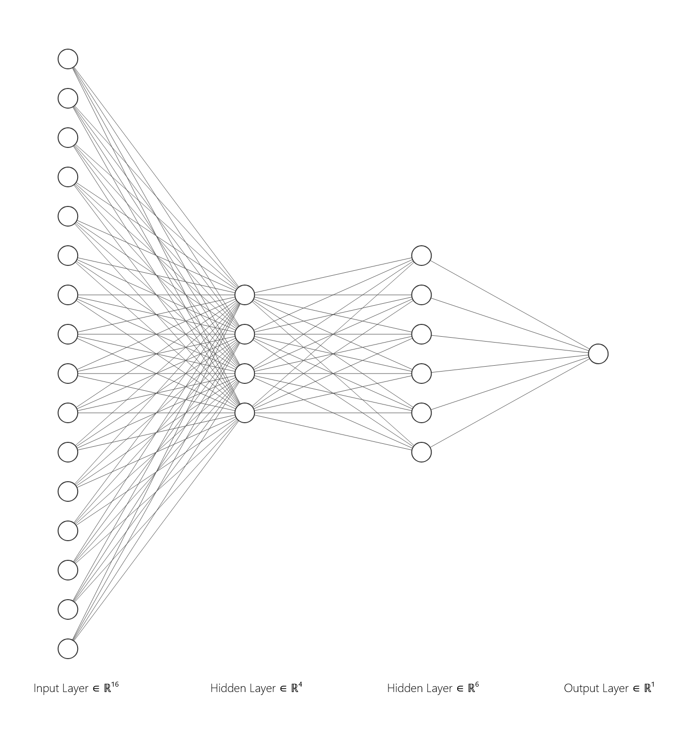
Simple MLP to fit flow, given extruder history.
W/ Yuval Mamana
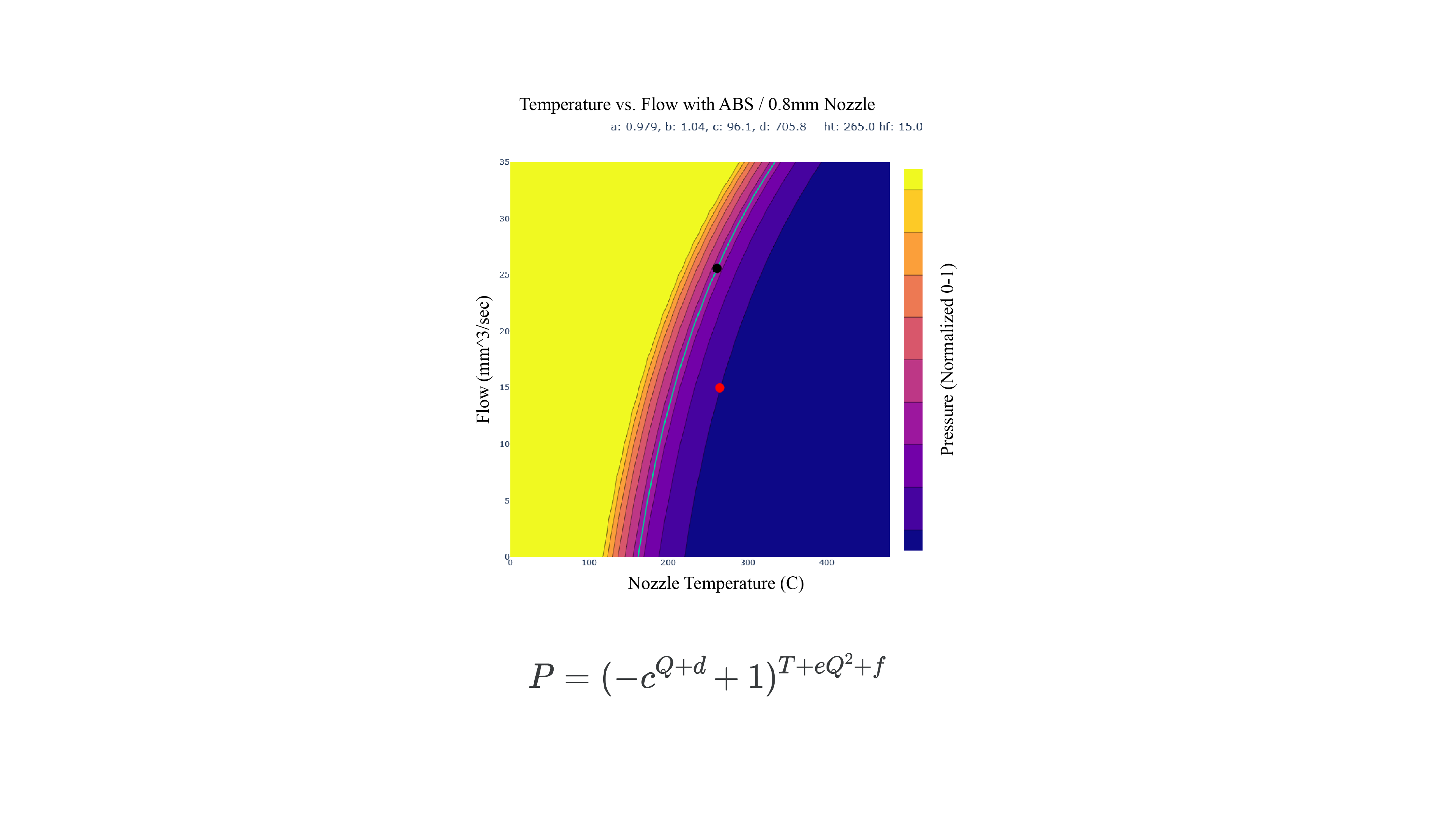
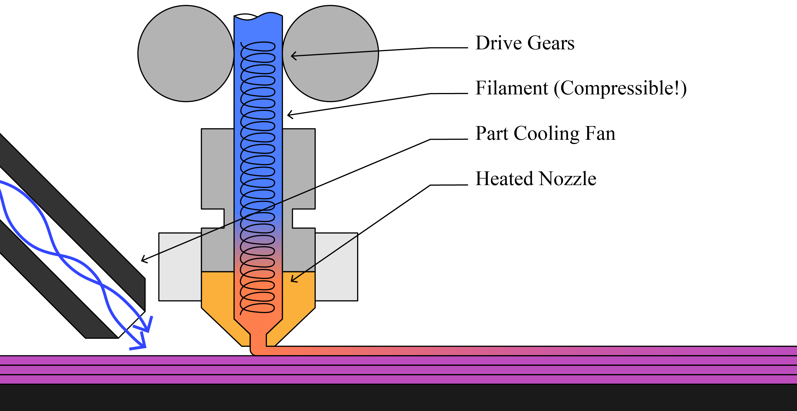
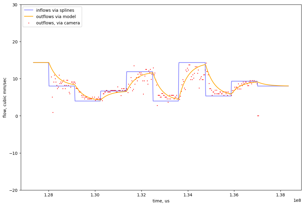
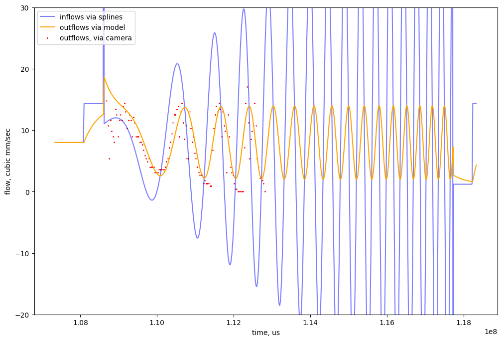
Simple Filament Compression Model
- $\dot{P} = Q_{in} - Q_{out}$
- $Q_{out} = Pk_{outflow}$
- $F_{in} = Tk_{tq} - Pk_{pushback} - Q_{in}k_{fric}$
- $\dot{Q}_{in} = F_{in}$
- Values:
- $Q_{out}$ is outflow (at nozzle)
- $Q_{in}$ is inflow (at motor)
- $P$ is 'pressure' in the chamber: is equivalent here to cubic millimeters of un-extruded filament in the chamber
- $F_{in}, Q_{in}$ are force and velocity for the filament (at the motor)
- Parameters:
- $k_{outflow}$ relates pressure to flow (and could become a function)
- $k_{tq}$ scales torque
- $k_{pushback}$ relates pressure to force (at motor)
- $k_{fric}$ is classic damping friction on the filament
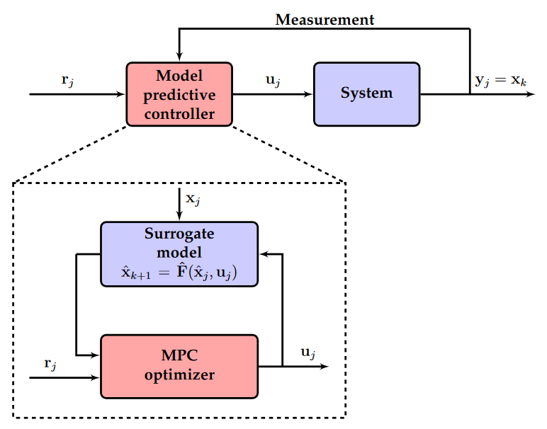
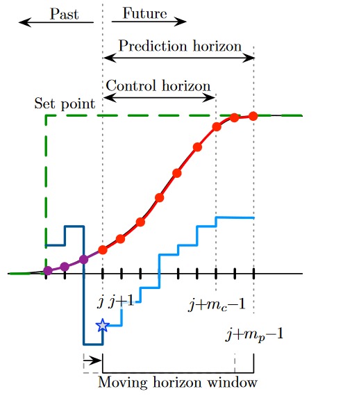
Brunton, Steven L, and J Nathan Kutz. 2022a. “Chapter 10: Data Driven Control.” In Data-Driven
Science and Engineering: Machine Learning, Dynamical Systems, and Control, 389-408. Cambridge,
United Kingdom: Cambridge University Press.
Di Carlo, Jared, Patrick M Wensing, Benjamin Katz, Gerardo Bledt, and Sangbae Kim. 2018. “Dynamic Locomotion in the Mit Cheetah 3 Through Convex Model-Predictive Control.” In 2018 IEEE/RSJ International Conference on Intelligent Robots and Systems (IROS), 1-9. IEEE.
Torrente, Guillem, Elia Kaufmann, Philipp Föhn, and Davide Scaramuzza. 2021. “Data-Driven MPC for Quadrotors.” IEEE Robotics and Automation Letters 6 (2): 3769-76.
Kuindersma, Scott, Robin Deits, Maurice Fallon, Andrés Valenzuela, Hongkai Dai, Frank Permenter, Twan Koolen, Pat Marion, and Russ Tedrake. 2016. “Optimization-Based Locomotion Planning, Estimation, and Control Design for the Atlas Humanoid Robot.” Autonomous Robots 40: 429-55.
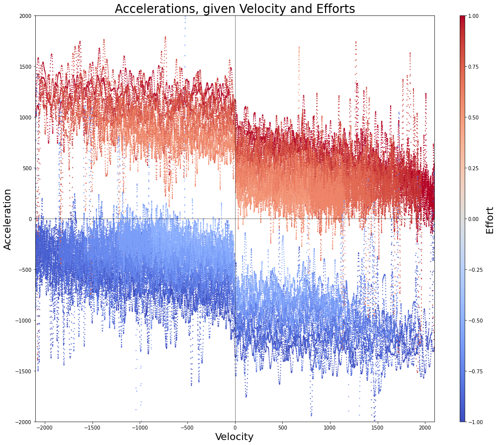
Definition of Forward Model for Motion
def integrate_pos(torques, vel, pos, del_t):
	params_torques = jnp.array([2000, 1000]) # motor juice per-axis
	params_frictional = jnp.array([2, 2])	 # damping

	torques = jnp.clip(torques, -1, 1)
	torques = torques * params_torques

	acc = torques - params_frictional * vel
	vel = vel + acc * del_t
	pos = pos + vel * del_t

	return acc, vel, pos
Definition of Forward Model for Polymer Flow
def integrate_flow(torque, inflow, pres, del_t):
	k_outflow = 2.85        # outflow = pres*k_outflow
	k_tq = 1                # torque scalar,
	k_pushback = 10         # relates pressure to torque
	k_fric = 0.2            # damping

	torque = np.clip(torque, -1, 1)

	# calculate force at top (inflow) and integrate for new inflow
	force_in = torque * k_tq - inflow * k_fric - np.clip(pres, 0, np.inf) * k_pushback
	inflow = inflow + force_in * del_t

	# outflow... related to previous pressure, is just proportional
	outflow = pres * k_outflow

	# pressure... rises w/ each tick of inflow, drops w/ outflow,
	pres = pres + inflow * del_t - outflow * del_t

	# that's all for now?
	return outflow, inflow, pres
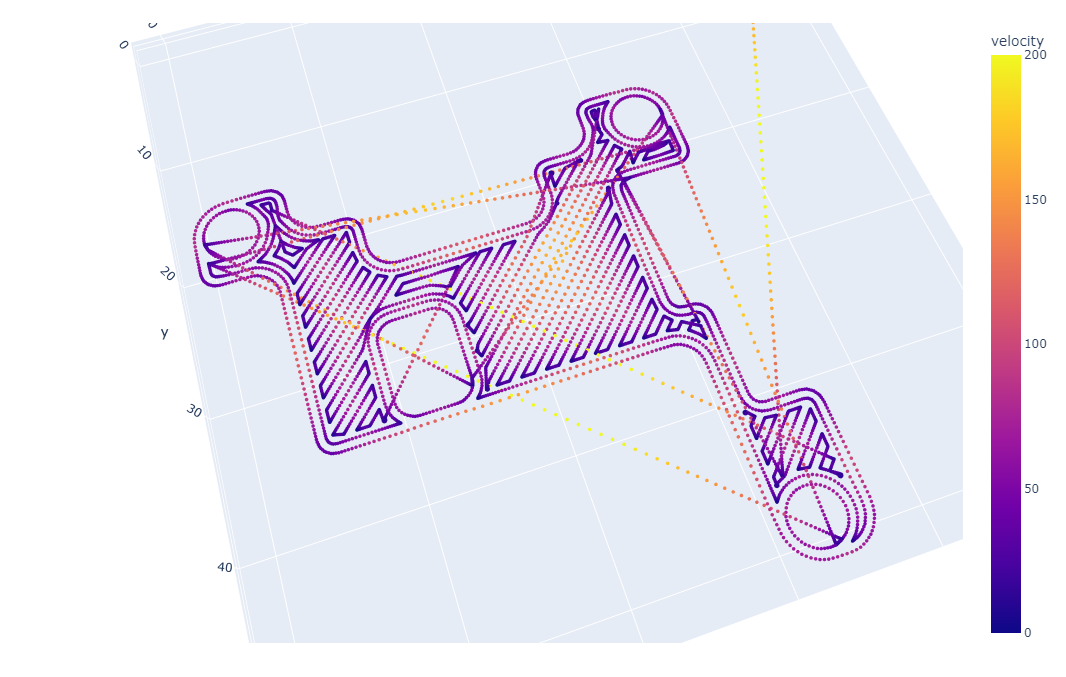
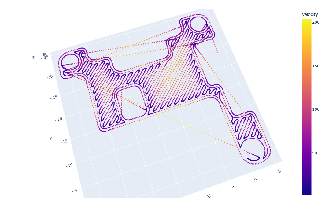
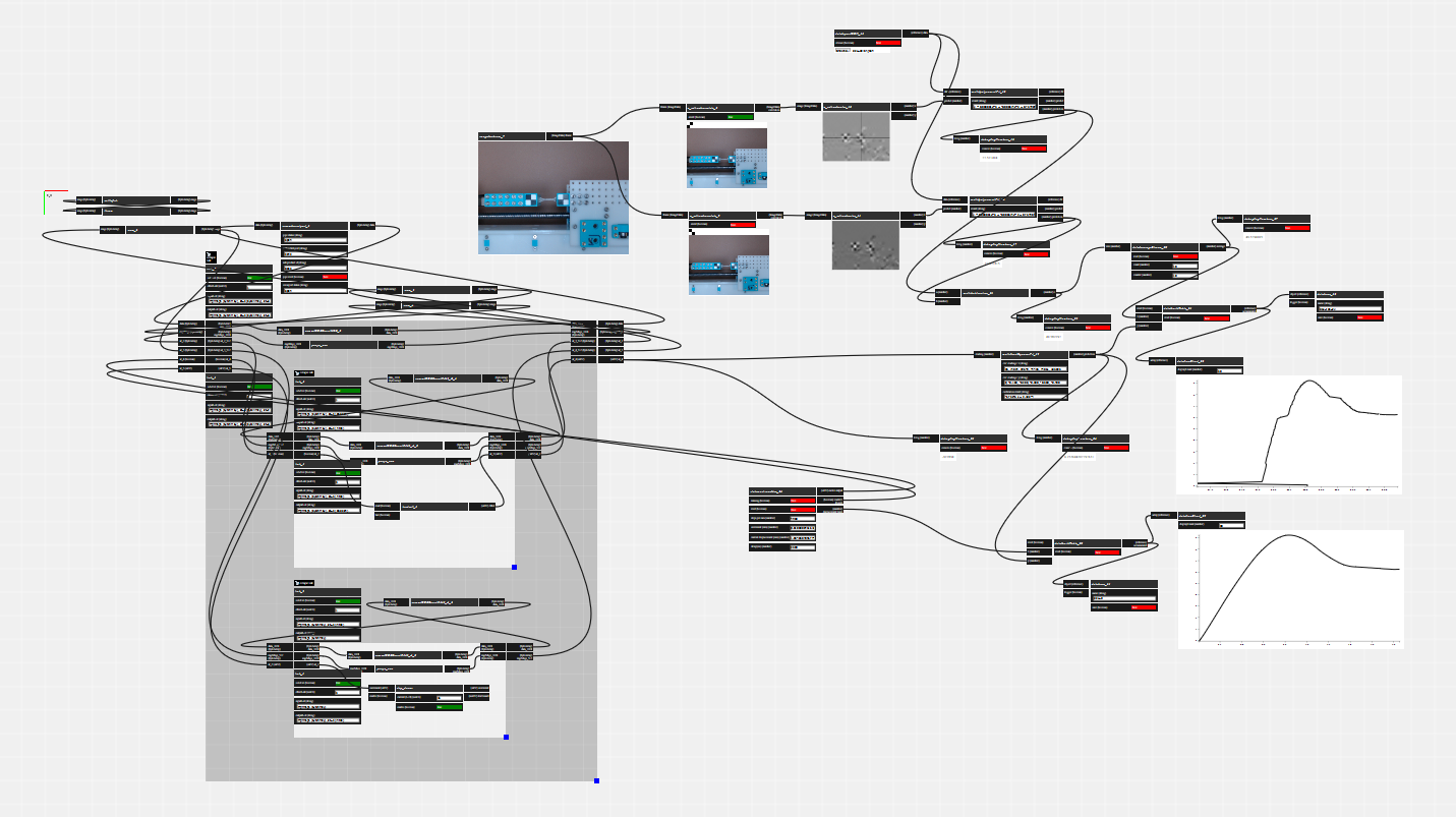
Optimizing path w/ compression model for extrusion (from data) and simple motor models.
Optimizing path w/ compression model for extrusion (from data) and simple motor models.
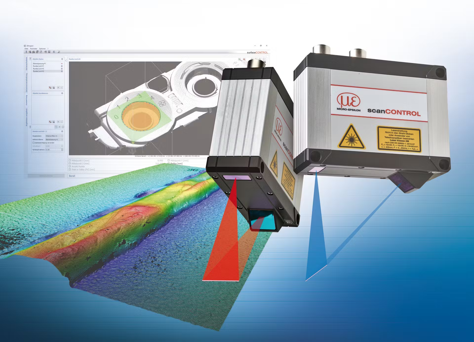
SOTA from Micro
Epsilon
Next Steps: per-layer model refinement via laser-scanned height maps.
Others deploying laser-line scanners for Printer calibration:
Wu, Pinyi. 2024. “Modeling and Feedforward Deposition Control in Fused Filament Fabrication.”
Abbot, Mike. 2023. “Rubedo: A System for Automatically Calibrating Pressure Advance Using Laser Triangulation.” https://github.com/furrysalamander/rubedo.
Wu, Pinyi. 2024. “Modeling and Feedforward Deposition Control in Fused Filament Fabrication.”
Abbot, Mike. 2023. “Rubedo: A System for Automatically Calibrating Pressure Advance Using Laser Triangulation.” https://github.com/furrysalamander/rubedo.
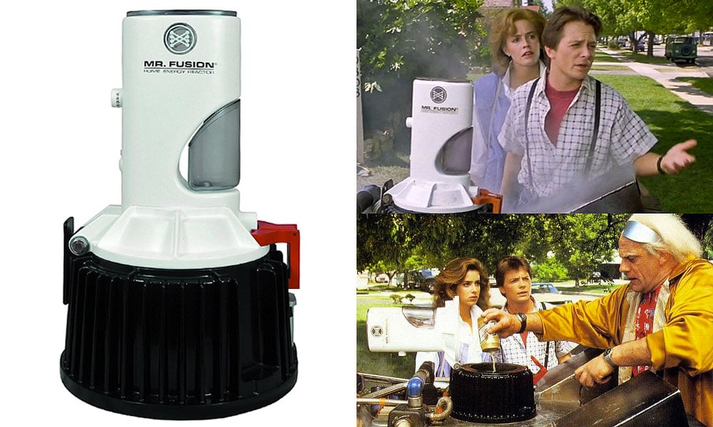
Recycled, Renewable, and Ad-Hoc
in Back to the Future
G21                   ; use millimeters
G28                   ; run the homing routine
G92 X110 Y120 Z30     ; set current position to (110, 120, 30)
G0  X10 Y10 Z10 F6000 ; "rapid" in *units per minute*
M3  S5000             ; turn the spindle on, at 5000 RPM
G1  Z-3.5 F600        ; plunge from (10, 10, 10) to (10, 10, -3.5)
G1  X20               ; draw a square, go to the right,
G1  Y20               ; go backwards 10mm
G1  X10               ; go to the left 10mm
G1  Y10               ; go forwards 10mm
G1  Z10               ; go up to Z10, exiting the material
M5                    ; stop the spindle
G0  X110 Y120 Z30     ; return to the position after homing (at 6000)
A simple GCode program, for a milling machine.
From Formation Plastics.
Built Up Edge (BUE) Formation, via YouTube.
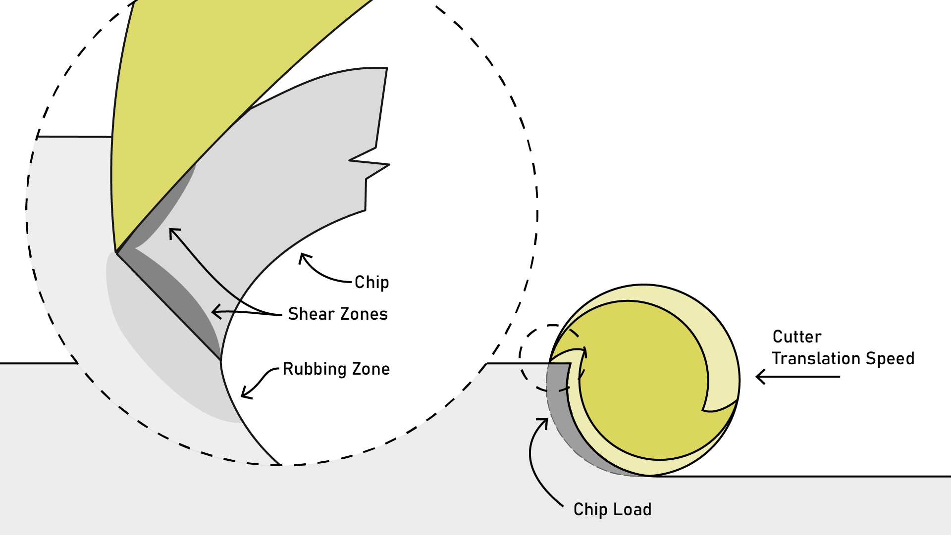
Schmitz, Tony L, and K Scott Smith. 2009. “Machining Dynamics.” Springer, 303.

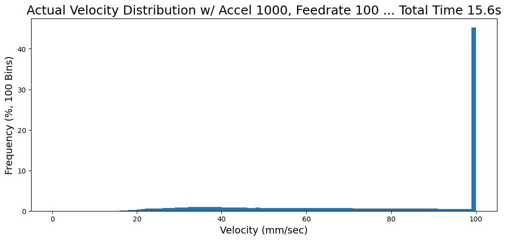
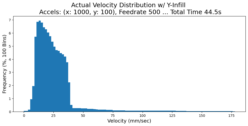
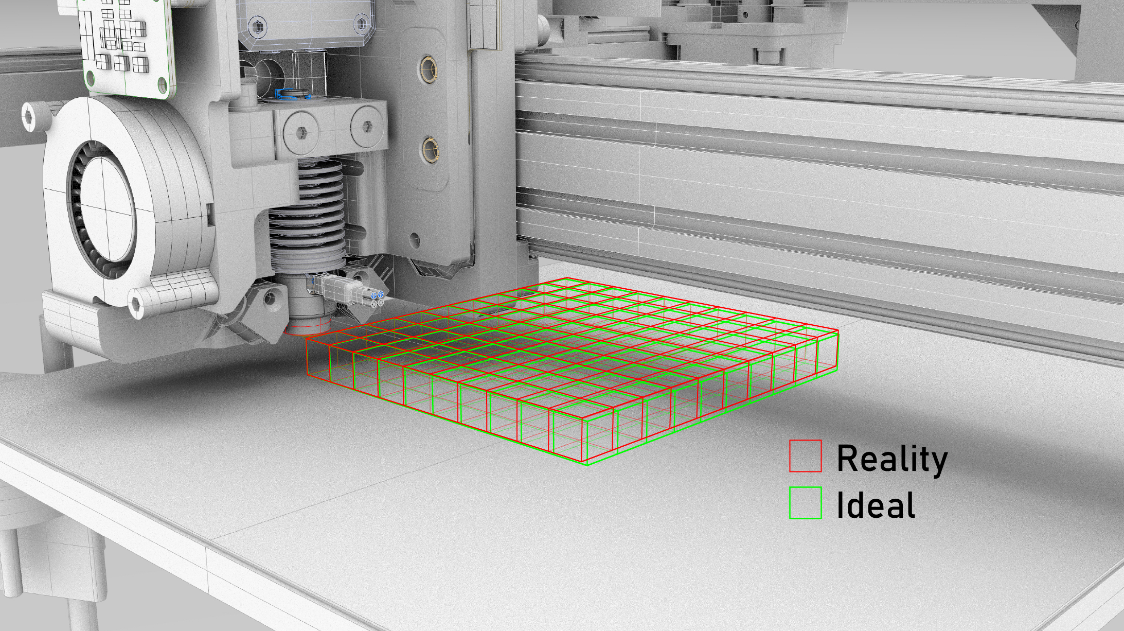
100mm/sec Feedrate Parameter,
1000mm/sec2 Acceleration Limit
1000mm/sec2 Acceleration Limit
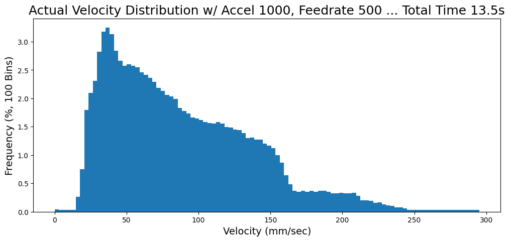
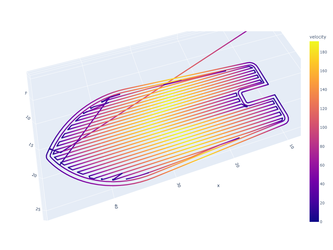
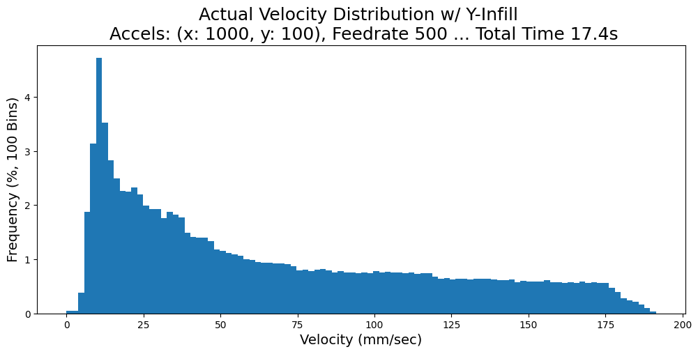
500mm/sec Feedrate Parameter
1000mm/sec2 Acceleration Limit
1000mm/sec2 Acceleration Limit
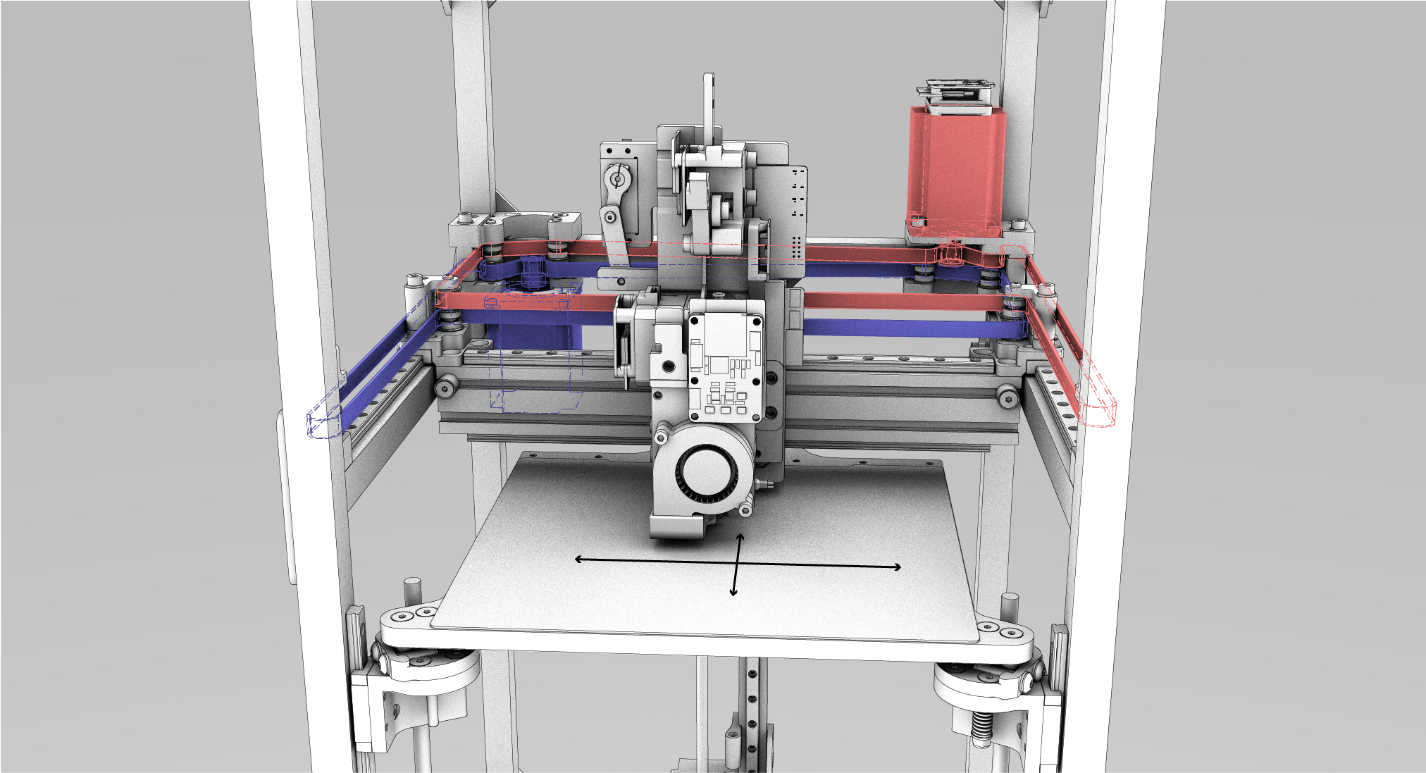
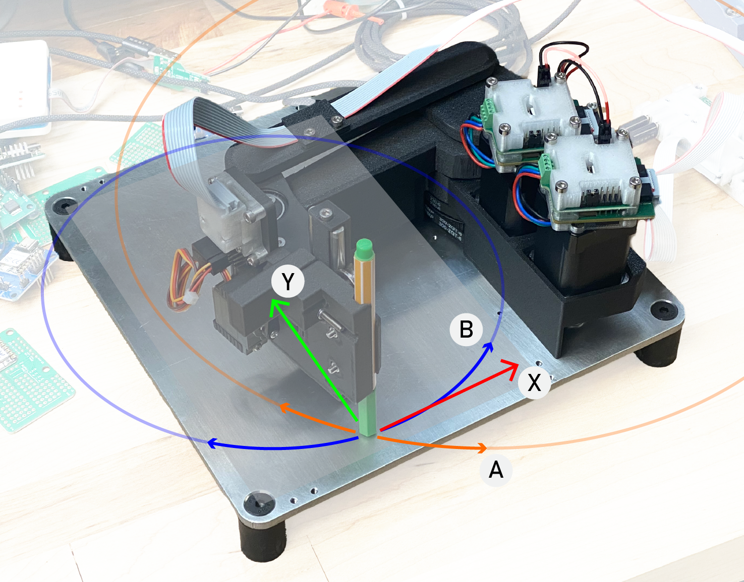
Moyer, Ilan. 2024. “CoreXY: A Mechanism for Motion Control in 3D Printers and CNC Machines.” https://corexy.com/.
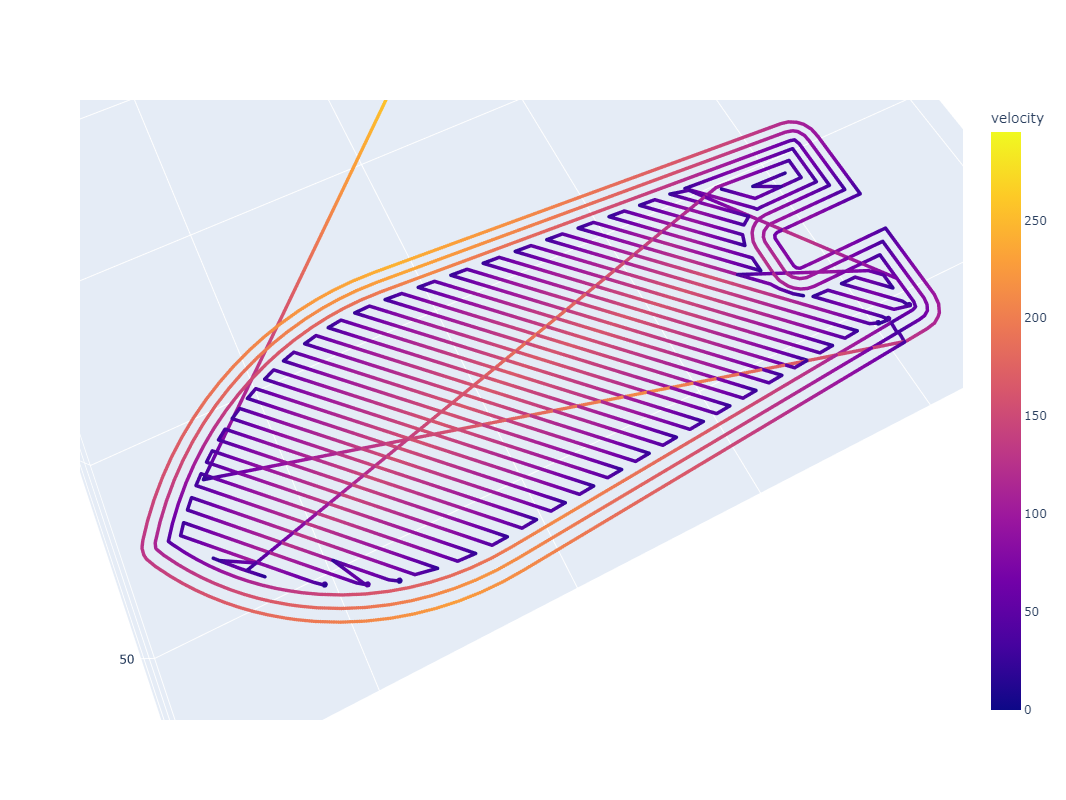
Motion Perpendicular to Dominant Axis
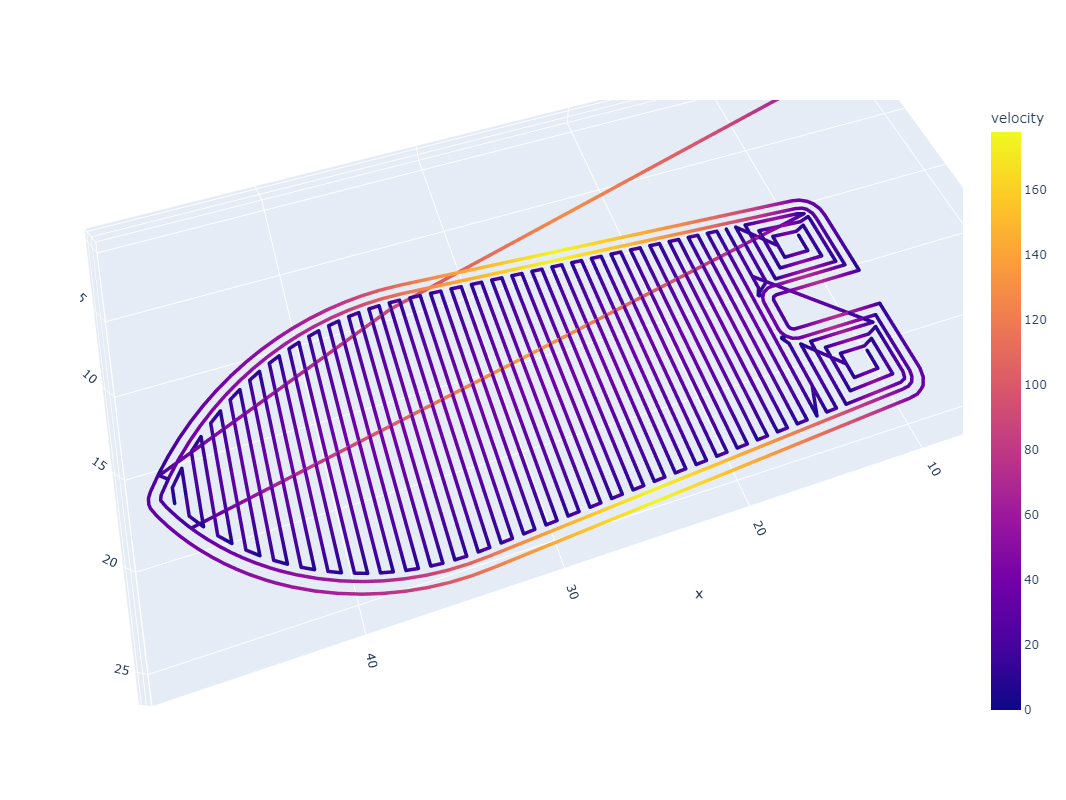
Motion Aligned to Dominant Axis
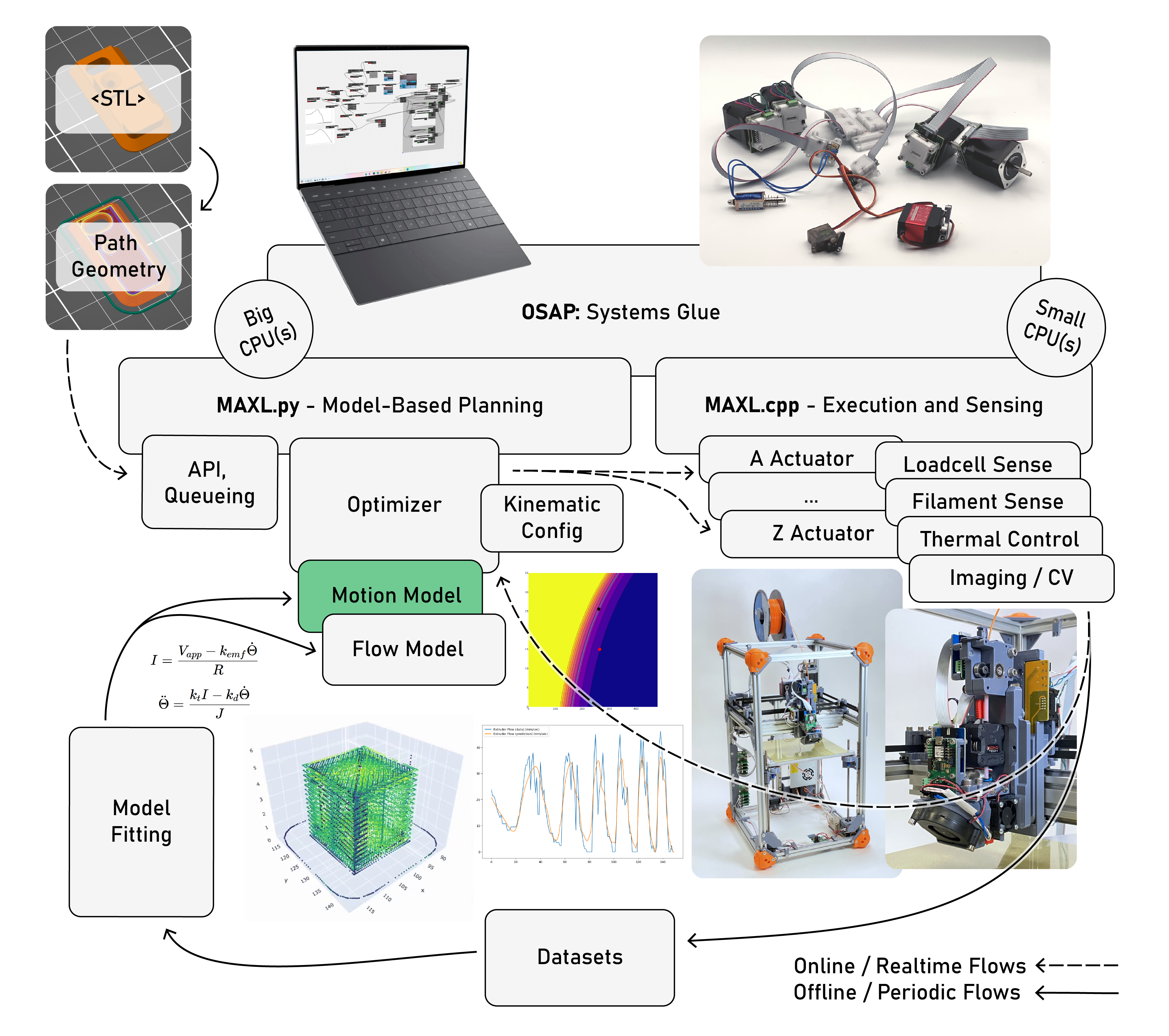
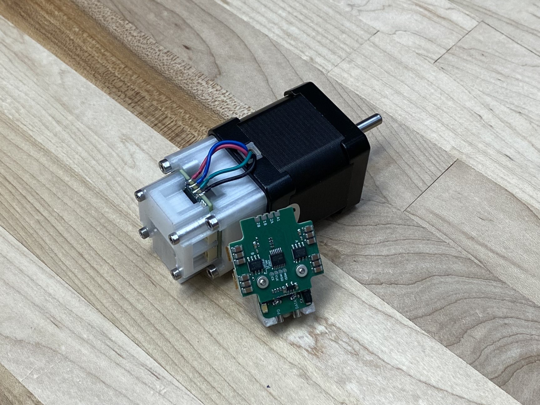
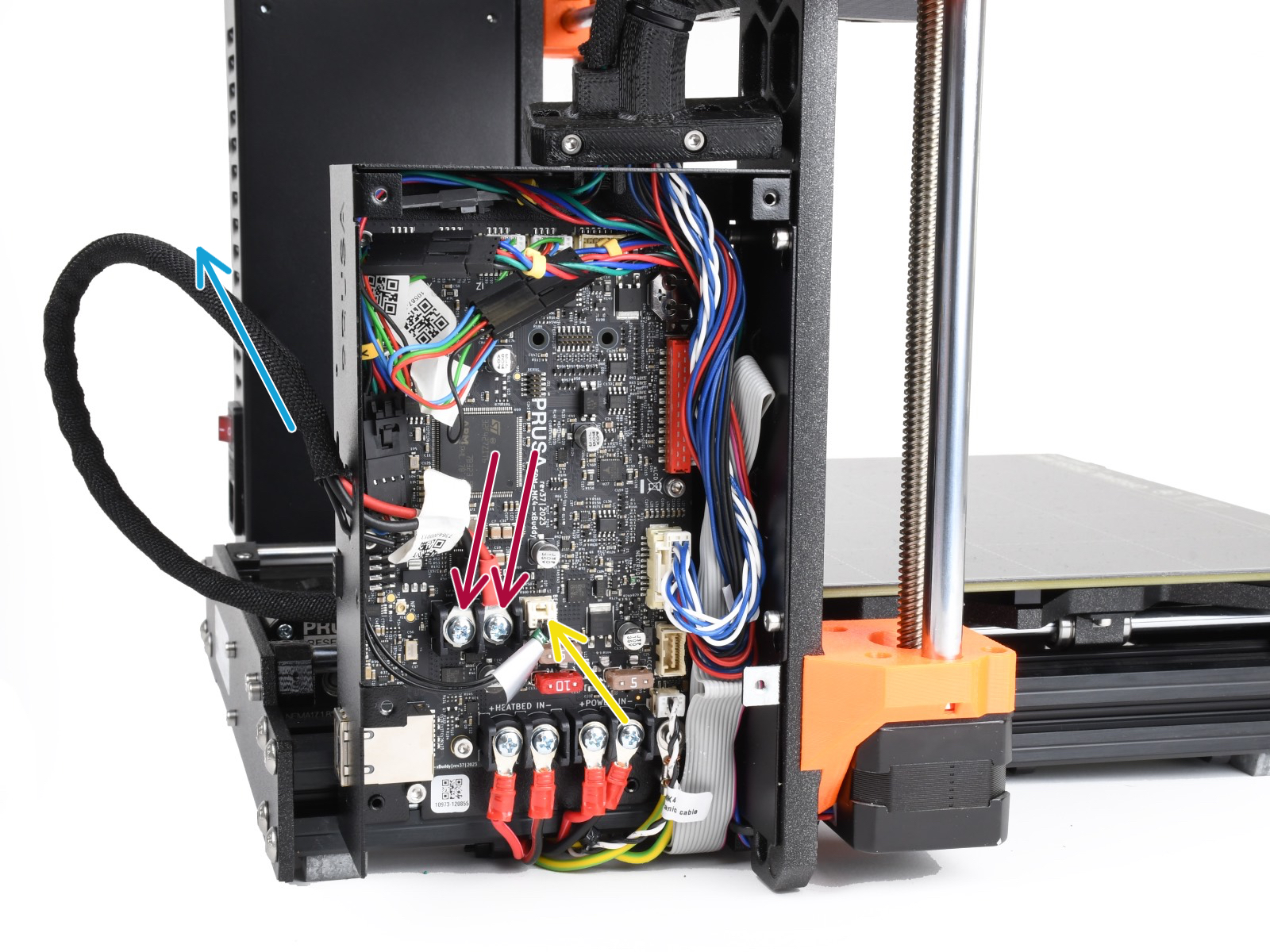
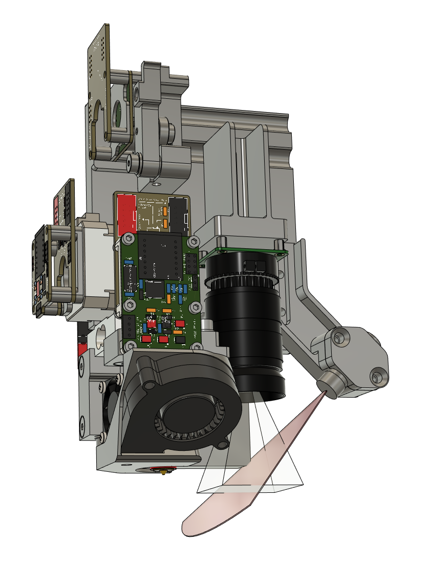
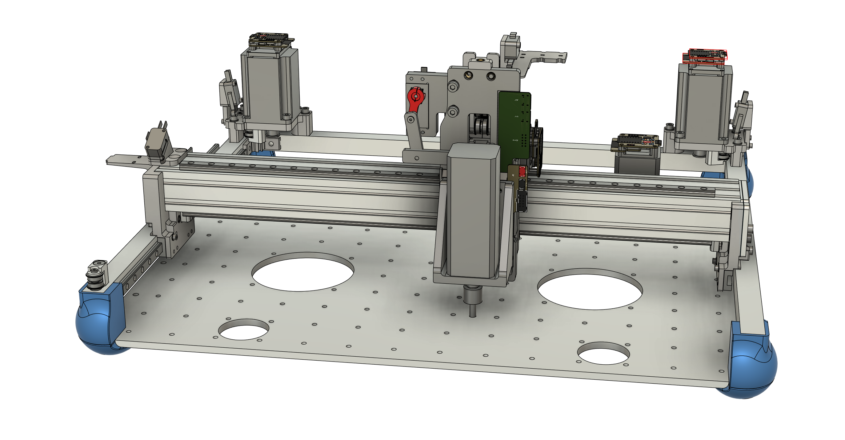
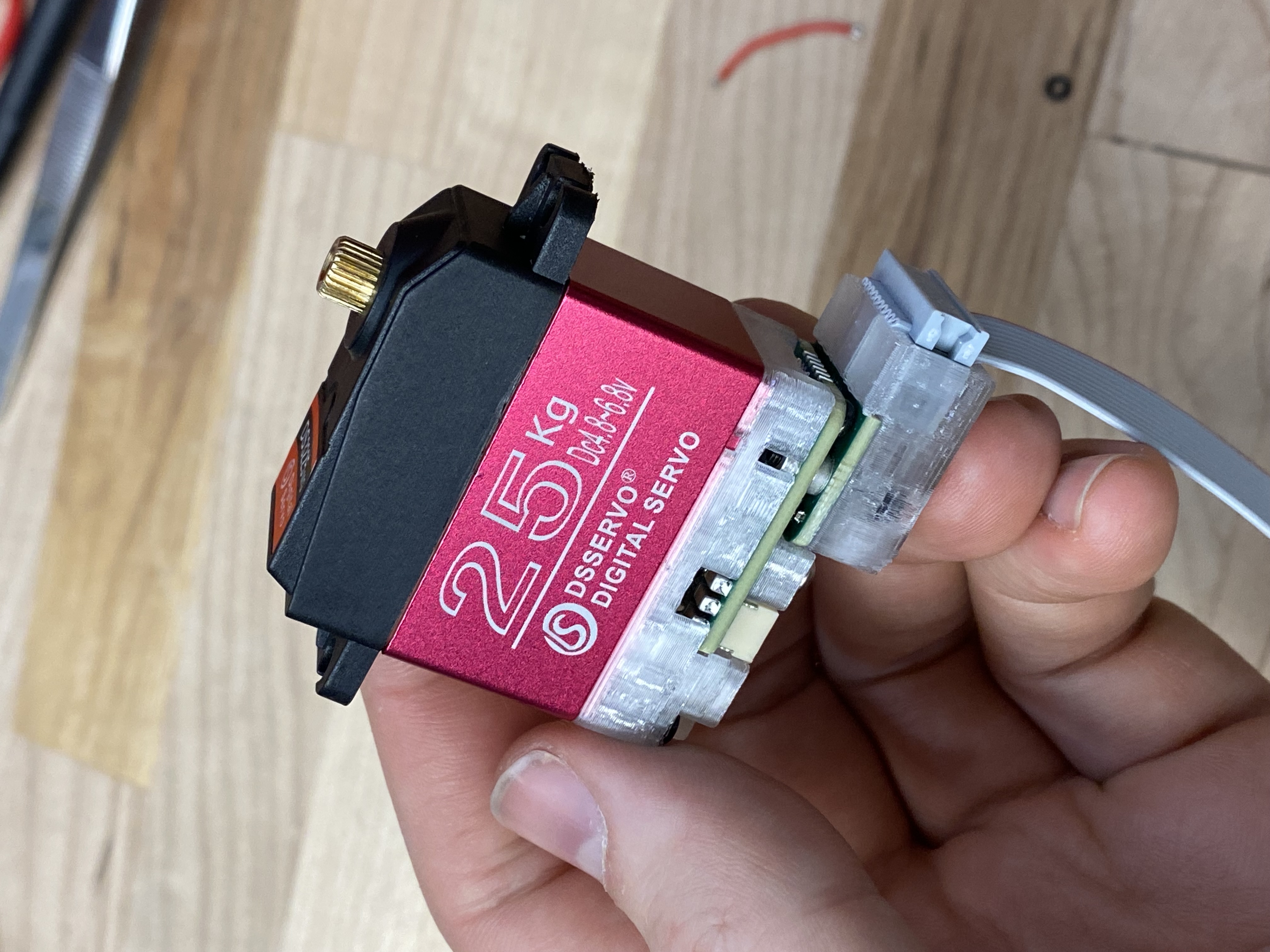
Closed-Loop Stepper Driver w/ 14-bit Encoder and Current Measurement
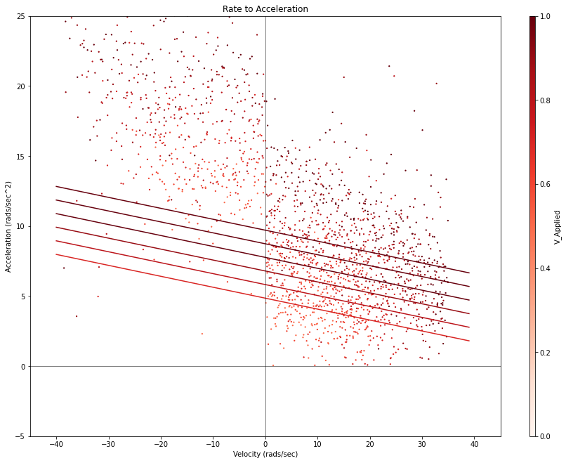
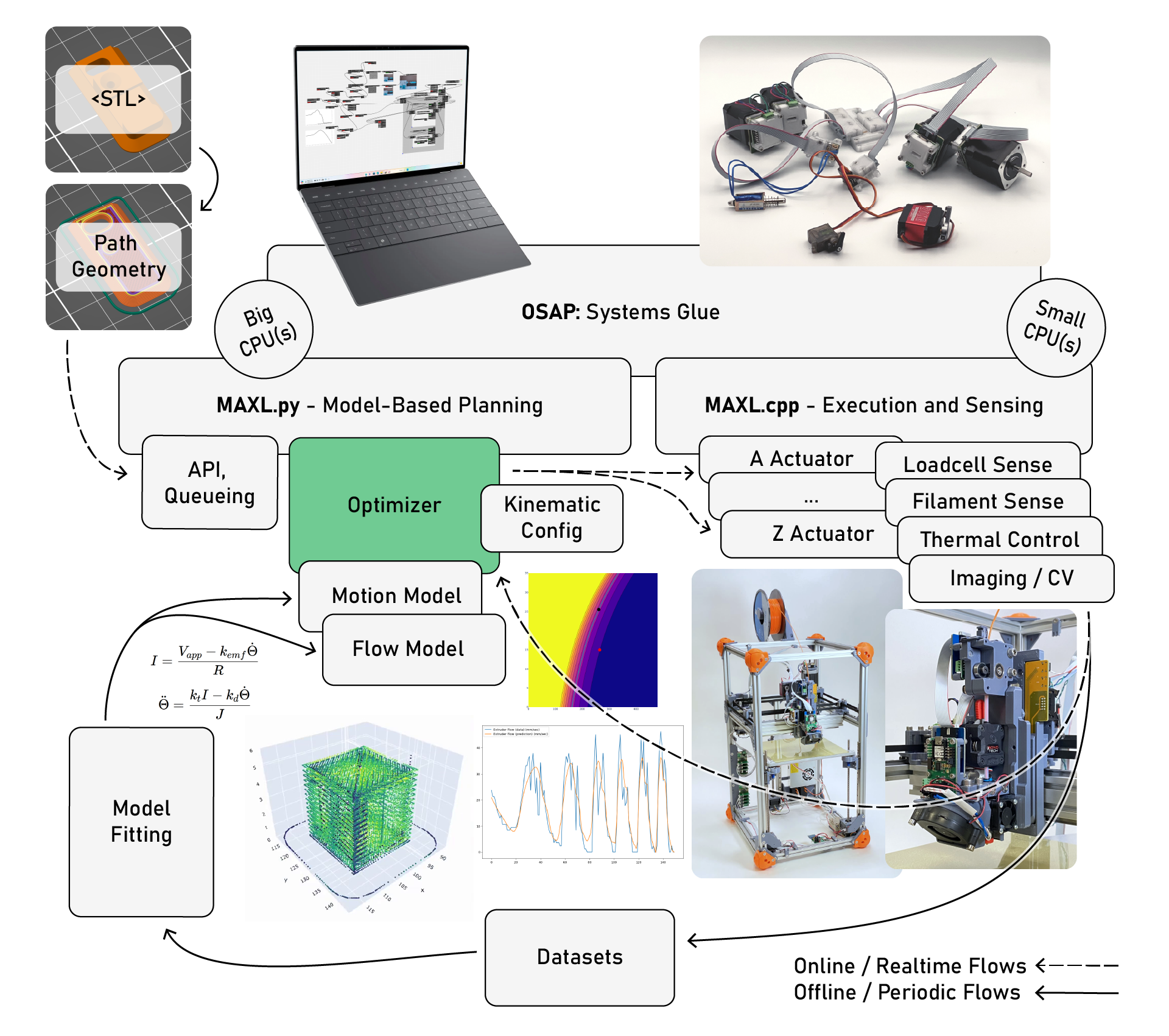
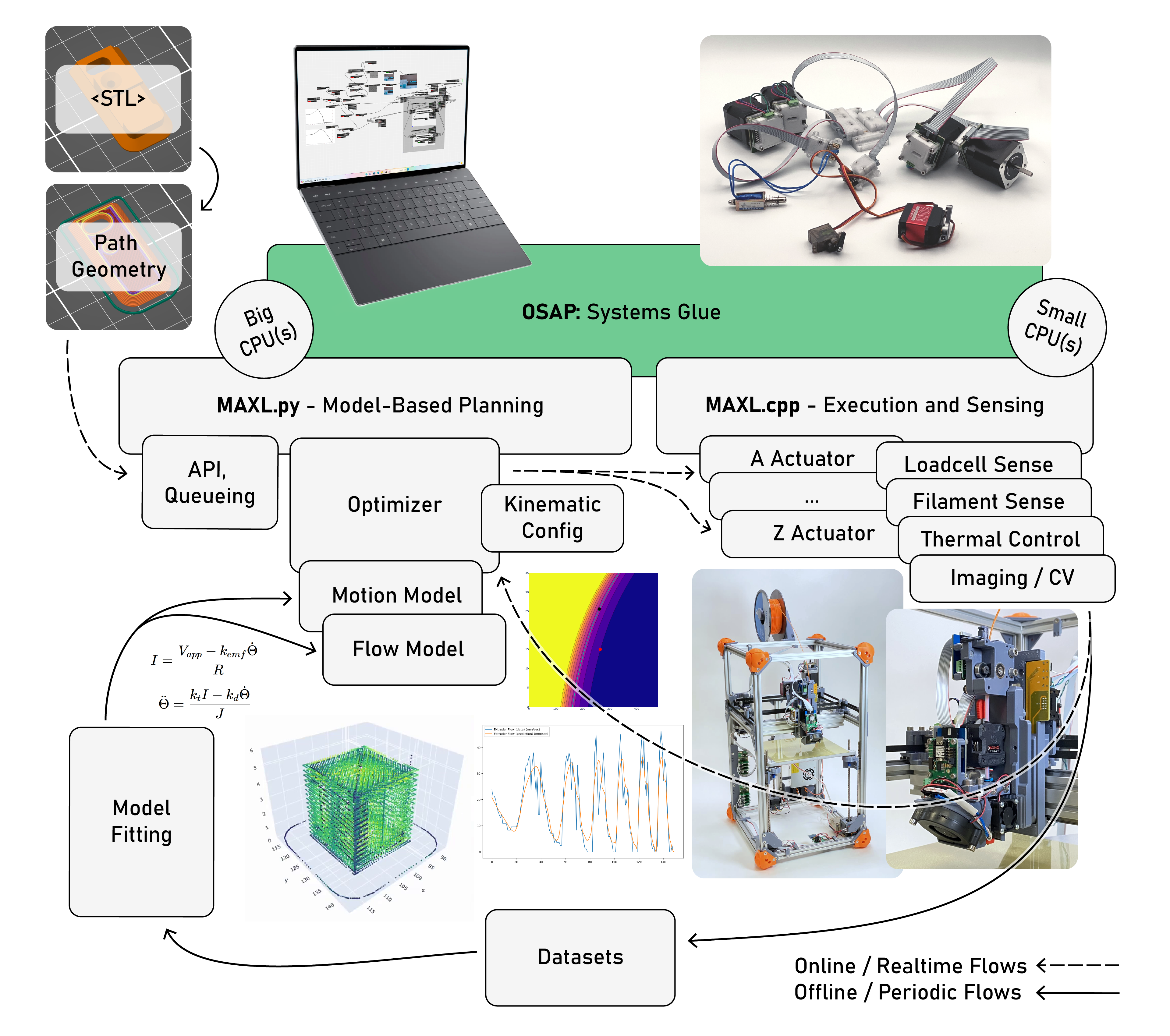
$$I = \frac{V_{app} - k_{emf}\dot{\Theta}}{R}$$
$$\ddot{\Theta} = \frac{k_tI - k_d\dot{\Theta}}{J}$$
Optimizing path w/ compression model for extrusion (from data) and simple motor models.
Path Solved with Trapezoids (common in SOTA)
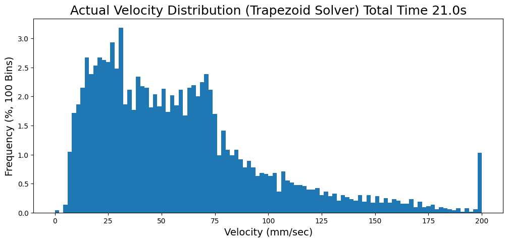
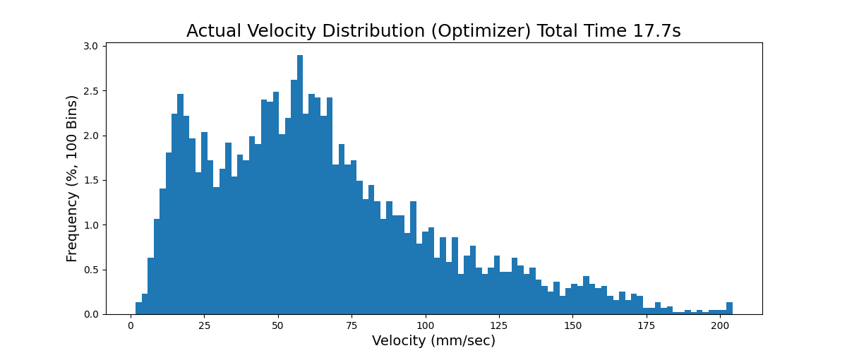
Path Solved with MPC (this work) (14% speedup)
Cutting Force per unit of Depth
$$F_t = K_{tc}ah(\theta) + K_{te}a$$
$$F_r = K_{rc}ah(\theta) + K_{re}a$$
$\theta$ is chip thickness$K_{tc}, K_{rc}$ are cutting force coefficients
$K_{te}, K_{re}$ are edge force coefficients
Dunwoody, Keith. Automated identification of cutting force coefficients and tool dynamics on
CNC machines. Diss. University of British Columbia, 2010.
Sharma, Chetan. Automatic modeling of machining processes. Diss. Massachusetts Institute of
Technology, 2021.
SOTA Resonance Testing
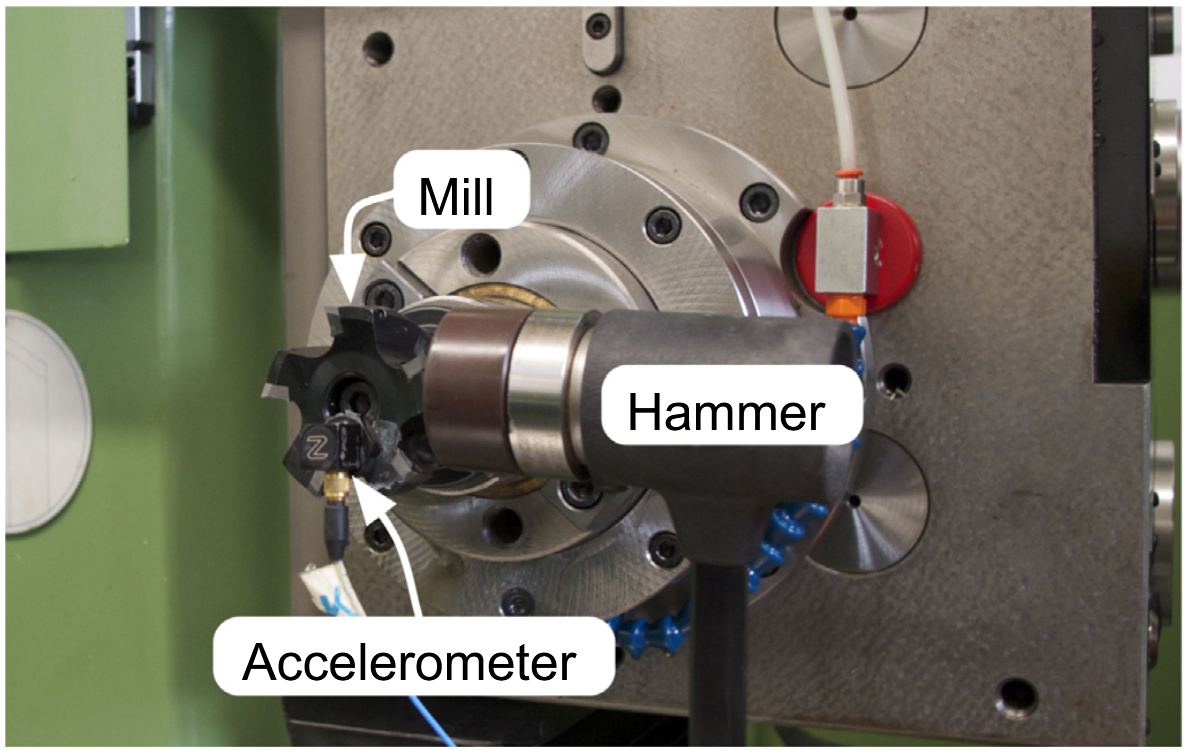
Bort, Carlos Maximiliano Giorgio, Marco Leonesio, and Paolo Bosetti. "A model-based adaptive
controller for chatter mitigation and productivity enhancement in CNC milling machines."
Robotics and Computer-Integrated Manufacturing 40 (2016): 34-43.
... from publication in-progress
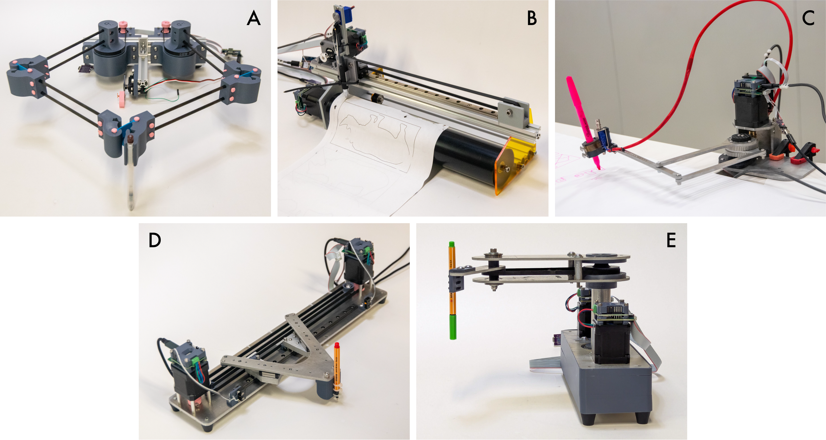
Plotter Comp 2025
Parameters:
January 28-31 @ MIT EDS Shop
4-6 Machine Builders
Materials and Controllers Provided
January 28-31 @ MIT EDS Shop
4-6 Machine Builders
Materials and Controllers Provided
Constraints:
Comp Regulation Pens (Stabilo Mini 88)
100x100mm Drawing Area
Comp Regulation Pens (Stabilo Mini 88)
100x100mm Drawing Area
Evaluation (Participants):
10x Comp Regulation SVG's
Speed
Precision
Accuracy
BOM Cost
Fabrication Complexity
10x Comp Regulation SVG's
Speed
Precision
Accuracy
BOM Cost
Fabrication Complexity
Evaluation (MAXL):
Heterogeneity of Kinematics
Performance
Ease of Setup
Inspectability, Debuggability, Extensibility
Heterogeneity of Kinematics
Performance
Ease of Setup
Inspectability, Debuggability, Extensibility
G21
G28
G92 X110 Y120 Z30
G0  X10 Y10 Z10 F6000
M3  S5000
G1  Z-3.5 F600
G1  X20
G1  Y20
G1  X10
G1  Y10
G1  Z10
M5
G0  X110 Y120 Z30
await machine.home()
machine.set_current_position([110, 120, 30])

await machine.goto_now([10, 10, 10], target_rate = 100)

await spindle.await_rpm(5000)

await machine.goto_via_queue([10, 10, -3.5], target_rate = 10)
await machine.goto_via_queue([20, 10, -3.5], target_rate = 10)
await machine.goto_via_queue([20, 20, -3.5], target_rate = 10)
await machine.goto_via_queue([20, 10, -3.5], target_rate = 10)
await machine.goto_via_queue([10, 10, 10], target_rate = 10)

await spindle.await_rpm(0)

await machine.goto_now([110, 120, 30], target_rate = 100)
The same basic program, articulated as GCode, or as calls to our Python API.
Moyer, Ilan Ellison. A gestalt framework for virtual machine control of automated tools. Diss.
Massachusetts Institute of Technology, 2013.
Peek, Nadya Meile. Making machines that make: object-oriented hardware meets object-oriented software. Diss. Massachusetts Institute of Technology, 2016.
Peek, Nadya Meile. Making machines that make: object-oriented hardware meets object-oriented software. Diss. Massachusetts Institute of Technology, 2016.
We can bottle complex routines into higher level APIs...
await machine.route_shape(svg = "target_file/file.svg", material = "plywood, 3.5mm")
And we can easily inspect some lower levels:
async def home(self, switch: Callable[[], Awaitable[Tuple[int, bool]]], rate: float = 20, backoff: float = 10):

	# move towards the switch at `rate`
	self.goto_velocity(rate)

	# await the switch signal
	while True:
		time, limit = await switch()
		if limit:
			# get the DOF's position as reconciled with the limit switch's actual trigger time
			states = self.get_states_at_time(time)
			pos_at_hit = states[0]
			# stop once we've hit the limit
			await self.halt()
			break
		else:
			await asyncio.sleep(0)

	# backoff from the switch
	await self.goto_pos_and_await(pos_at_hit + backoff)
Firmwares contain function implementations.
// in hbridge firmware
float readAvailableVCC(void){
	const float r1 = 10000.0F;
	const float r2 = 470.0F;
	// it's this oddball, no-init ADC stuff,
	// teensy is 10-bits basically, y'all
	uint16_t val = analogRead(PIN_SENSE_VCC);
	// convert to voltage,
	float vout = (float)(val) * (3.3F / 1024.0F);
	// that's at 10k - sense - 470r - gnd,
	// vout = (vcc x r2) / (r1 + r2)
	// (vout * (r1 + r2)) / r2 = vcc
	float vcc = (vout * (r1 + r2)) / r2;
	return vcc;
}

// one line to generate an interface
BUILD_RPC(readAvailableVCC, "", "");
We can access those from other contexts
via proxy classes.
# auto-generated proxy,
class HBridgeProxy:
	# ...
	async def read_available_vcc(self) -> float:
		result = await self._read_available_vcc_rpc.call()
		return cast(float, result)
	# ...
These interfaces are generated automatically, using information
provided by the firmware.
We can use those interfaces to author, debug and modify high-level logic without mucking
about in hardware.
# discover all devices
system_map = await osap.netrunner.update_map()

# build a proxy, check existence
hbridge = HbridgeSamd21DuallyProxy(osap, "hbridge_dually")
try:
	await hbridge.begin()
except NameError:
	print("no hbridge found, check connections...")

print("... request voltage")
await hbridge.set_pd_request_voltage(15)

print("... await voltage")
while True:
	vcc_avail = await hbridge.read_available_vcc()
	print(F"avail: ${vcc_avail:.2f}")
	if vcc_avail > 14.0:
		break

print("pulse...")
for _ in range(100):
	print("...")
	await hbridge.pulse_bridge(2.0, 1000)
	await asyncio.sleep(1.75)
	await hbridge.pulse_bridge(-1.0, 50)
	await asyncio.sleep(1)

print("... done!")
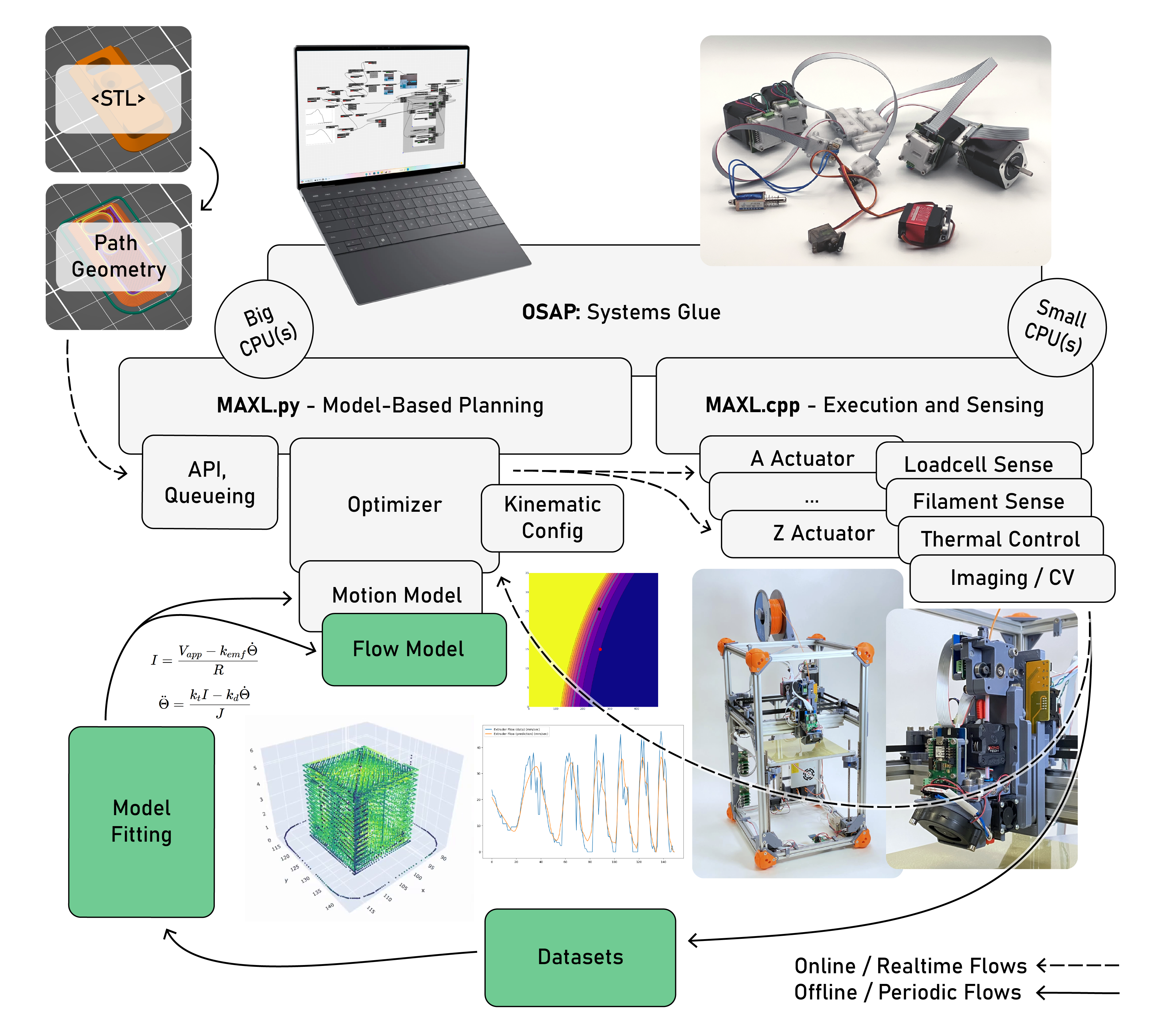
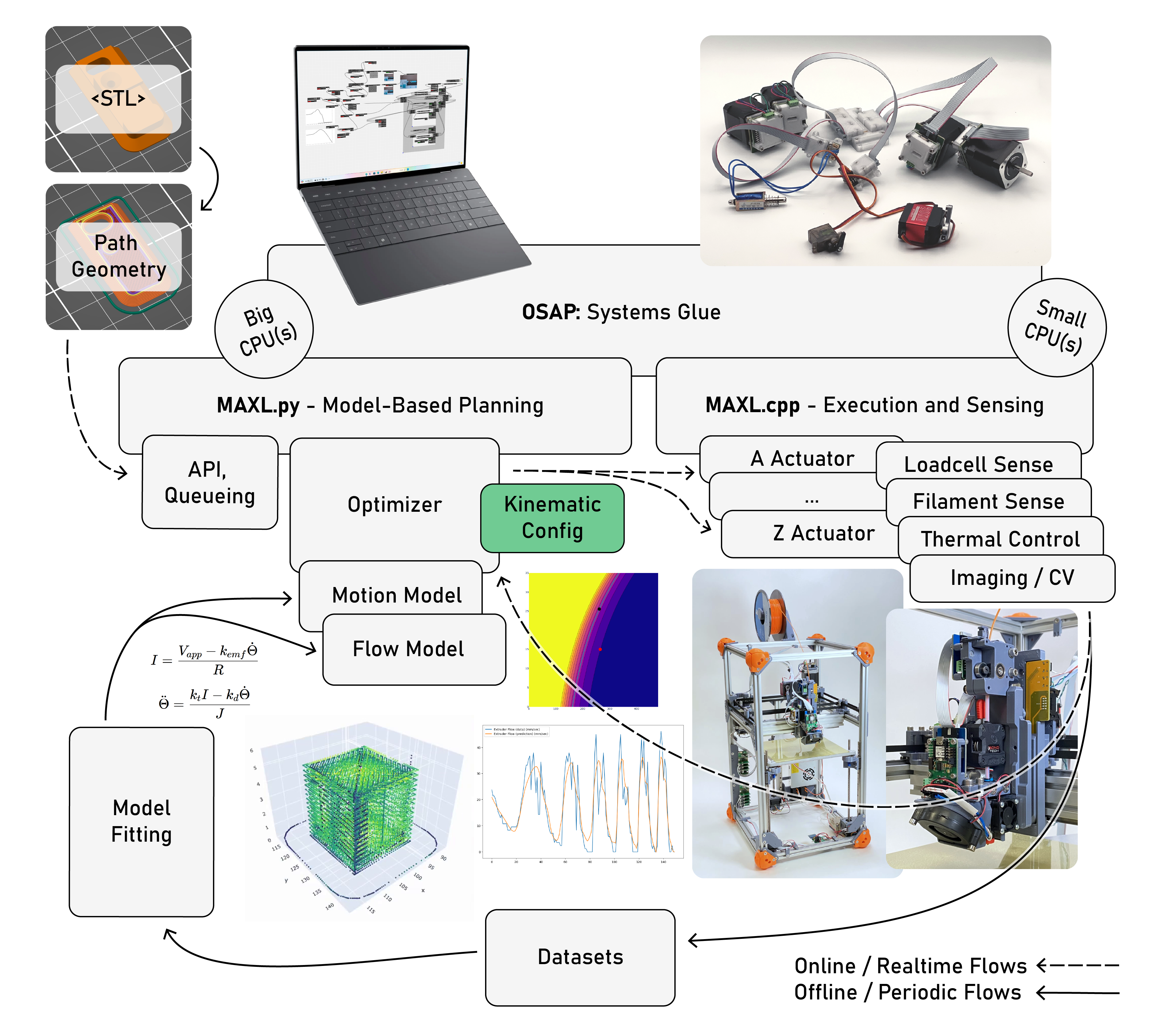
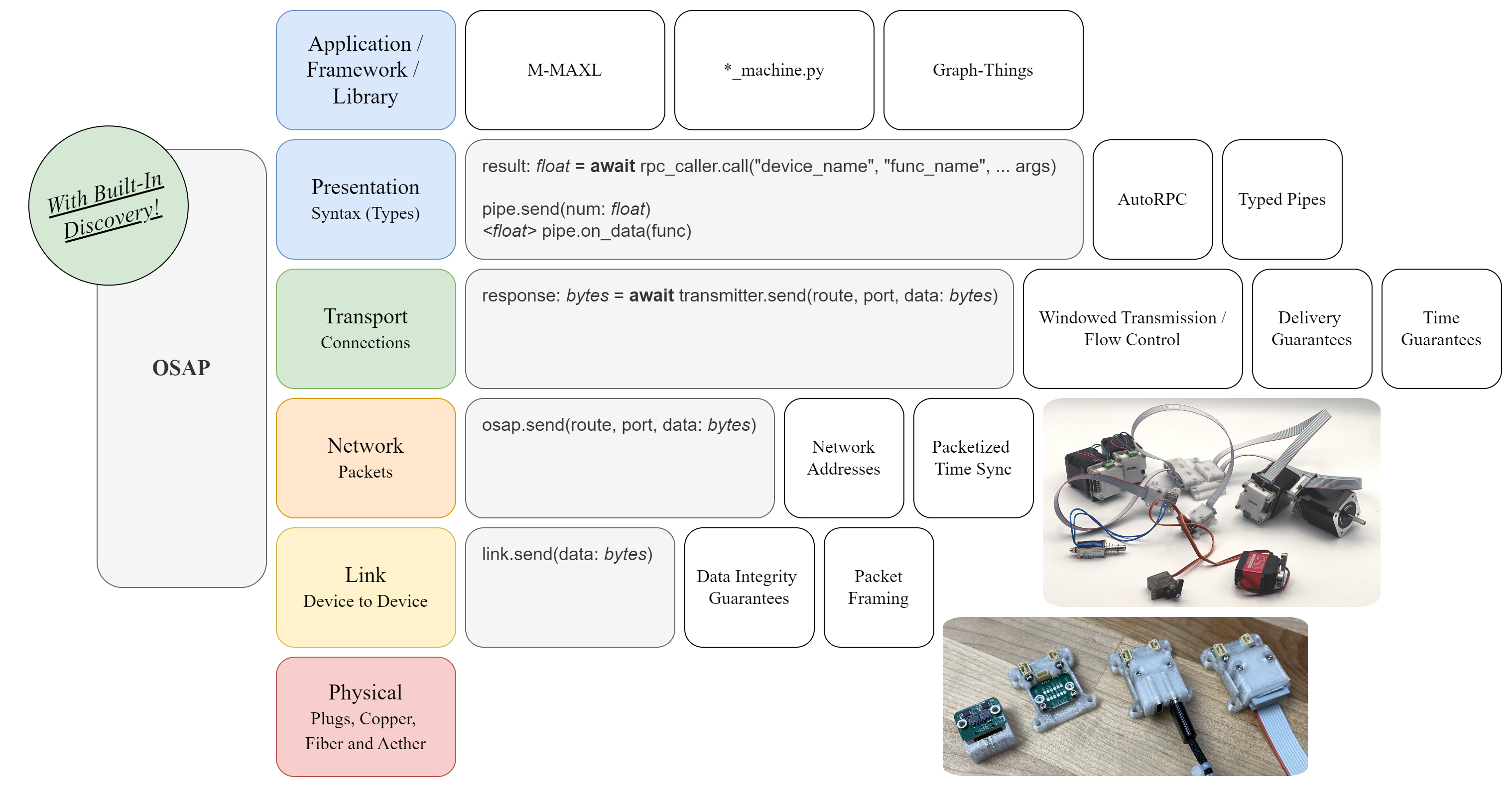
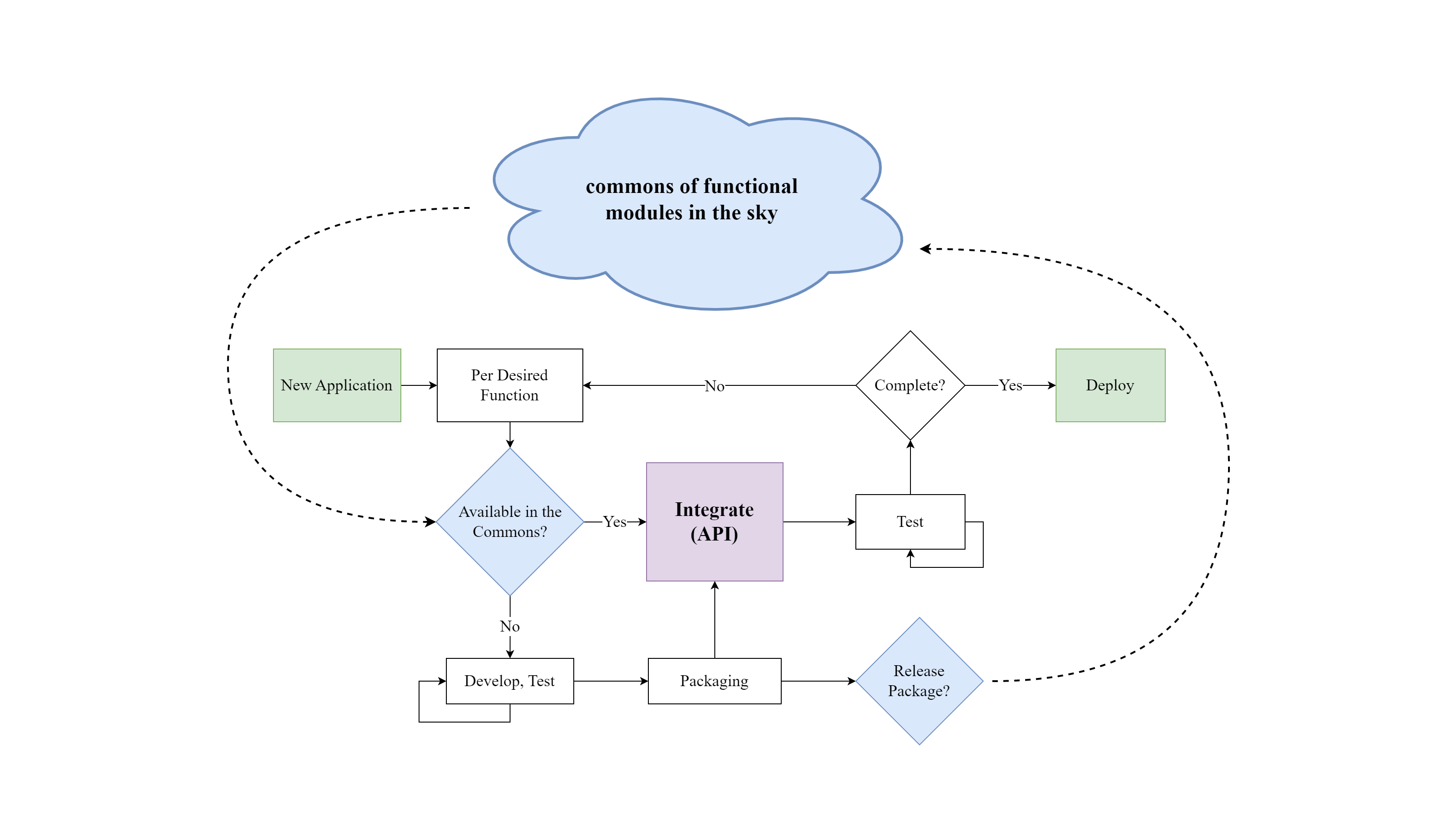
Automatic generation of software interfaces: single-source-of-truth, self-describing modular devices
for distributed systems.
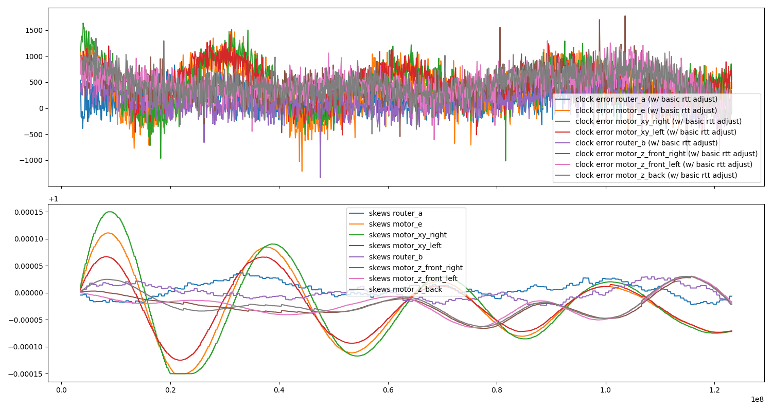
Distributed Clock Sync on 'any' Link: with under 1ms Error Target: 50us
Mills, David L. 1991. “Internet Time Synchronization: The Network Time Protocol.” IEEE Transactions on Communications 39 (10): 1482-93.
Eidson, John C, Mike Fischer, and Joe White. 2002. “IEEE-1588™ Standard for a Precision Clock Synchronization Protocol for Networked Measurement and Control Systems.” In Proceedings of the 34th Annual Precise Time and Time Interval Systems and Applications Meeting, 243-54.
Ciuffoletti, Augusto. "Using simple diffusion to synchronize the clocks in a distributed system." 14th International Conference on Distributed Computing Systems. IEEE, 1994.
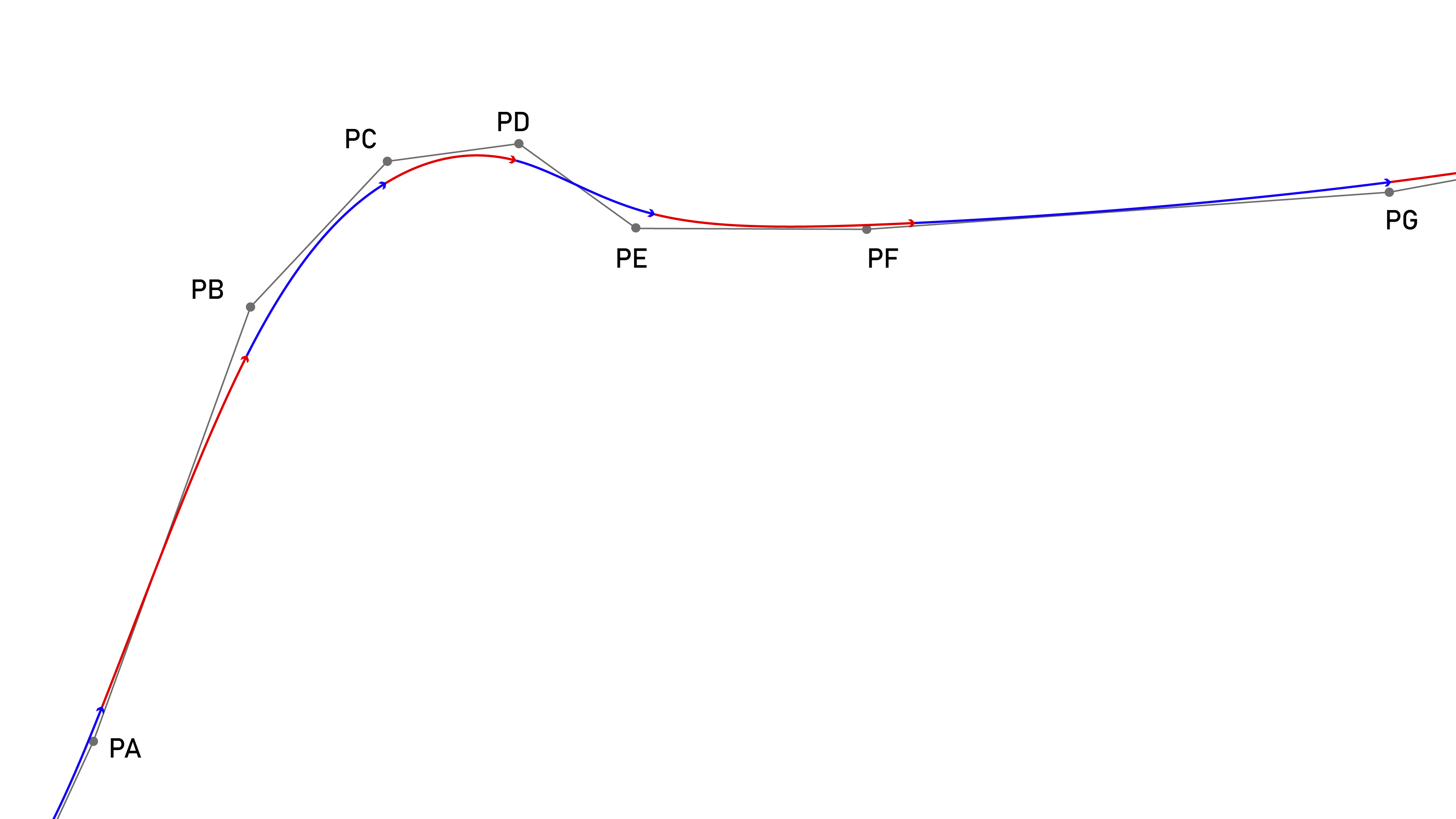
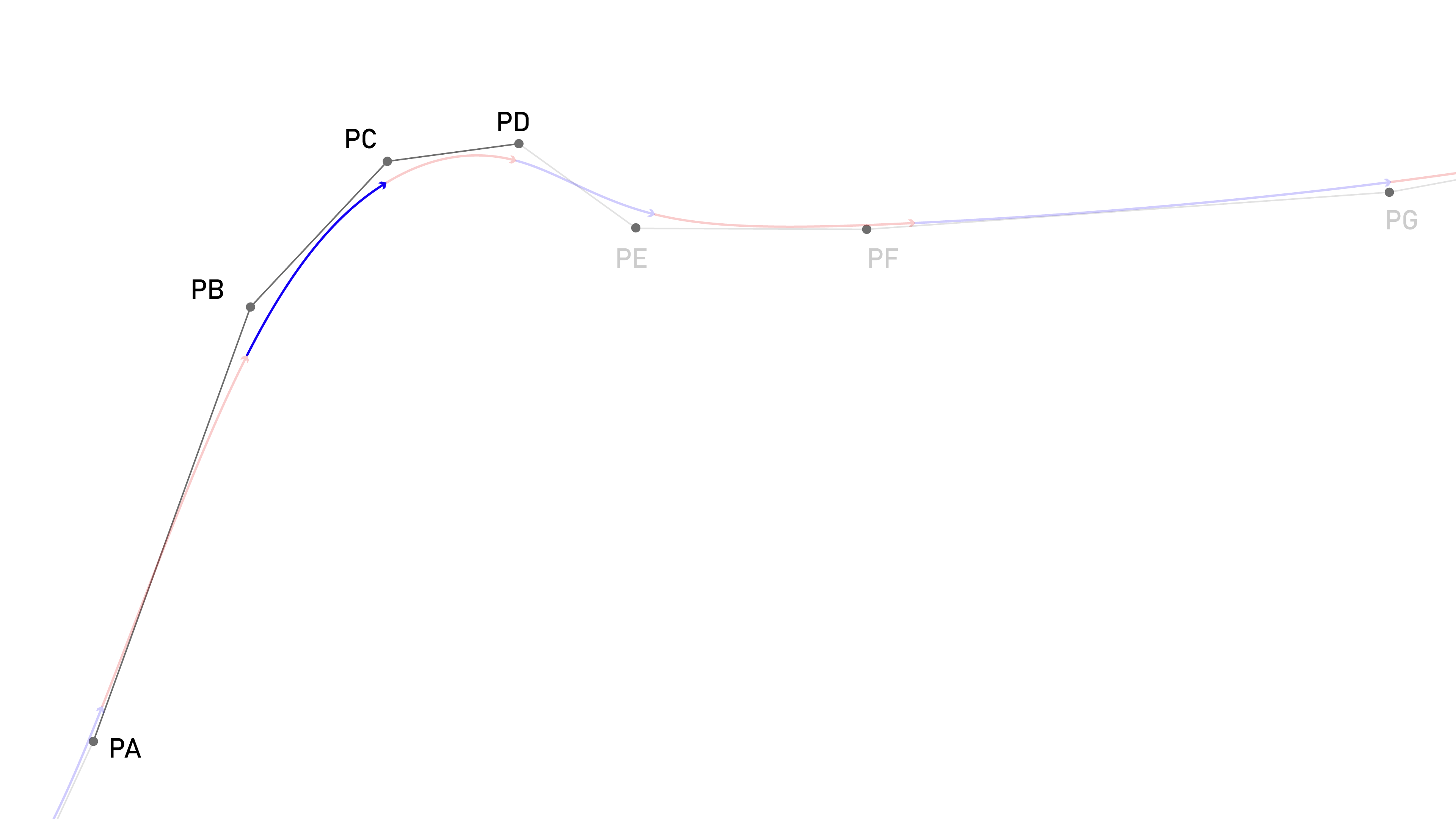
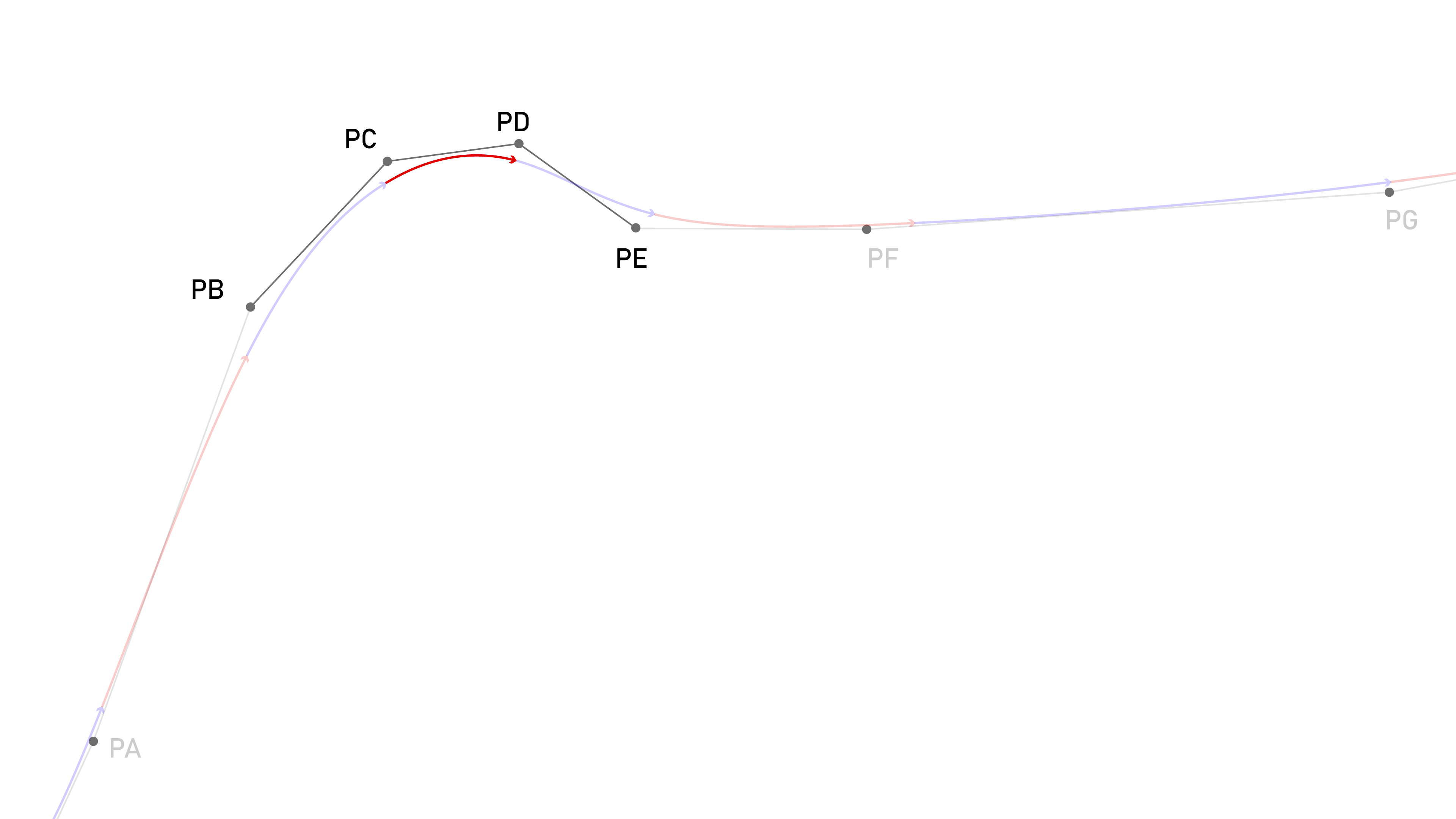
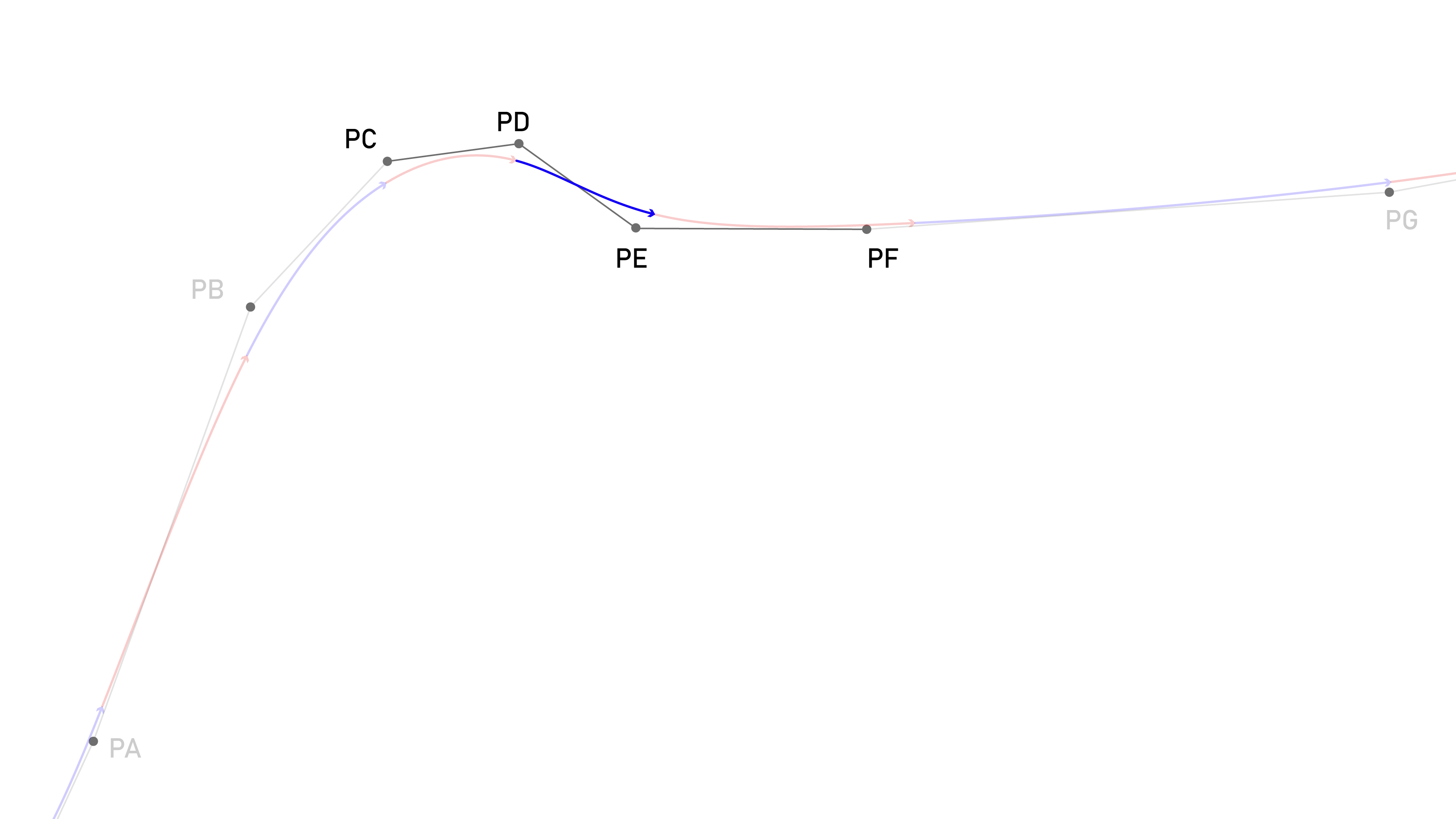
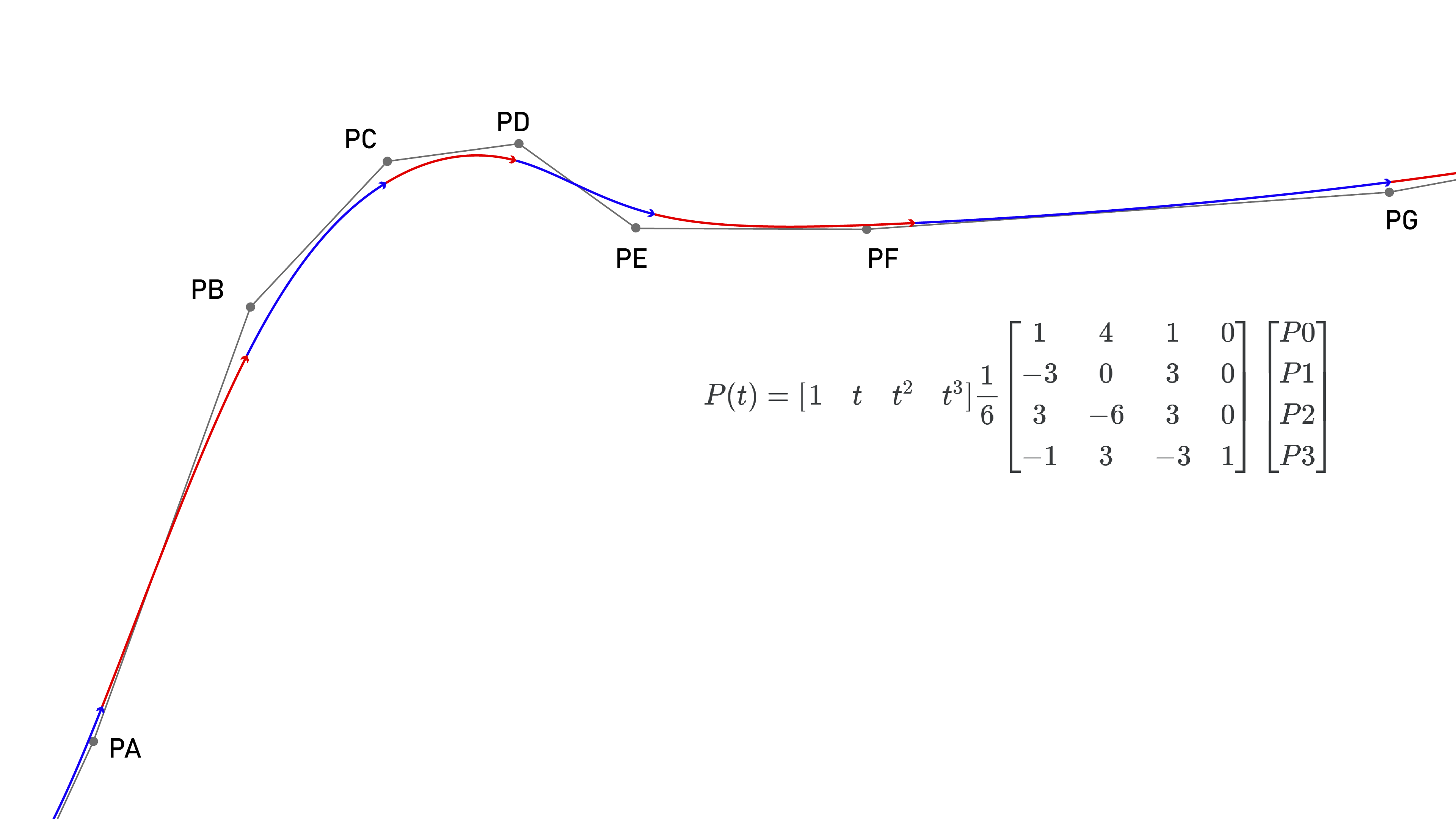
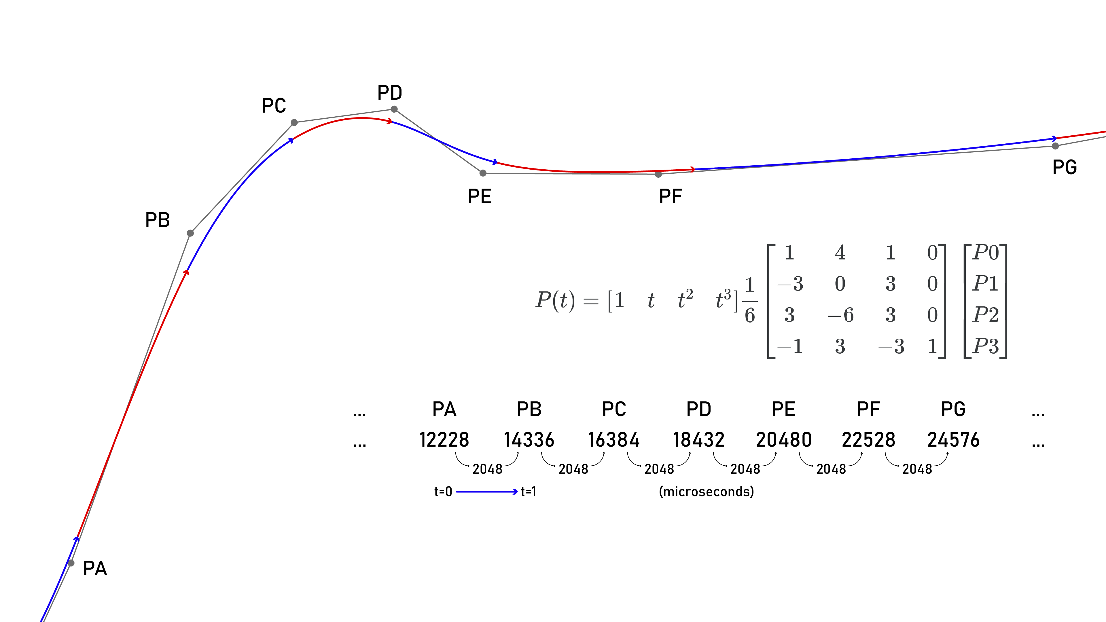
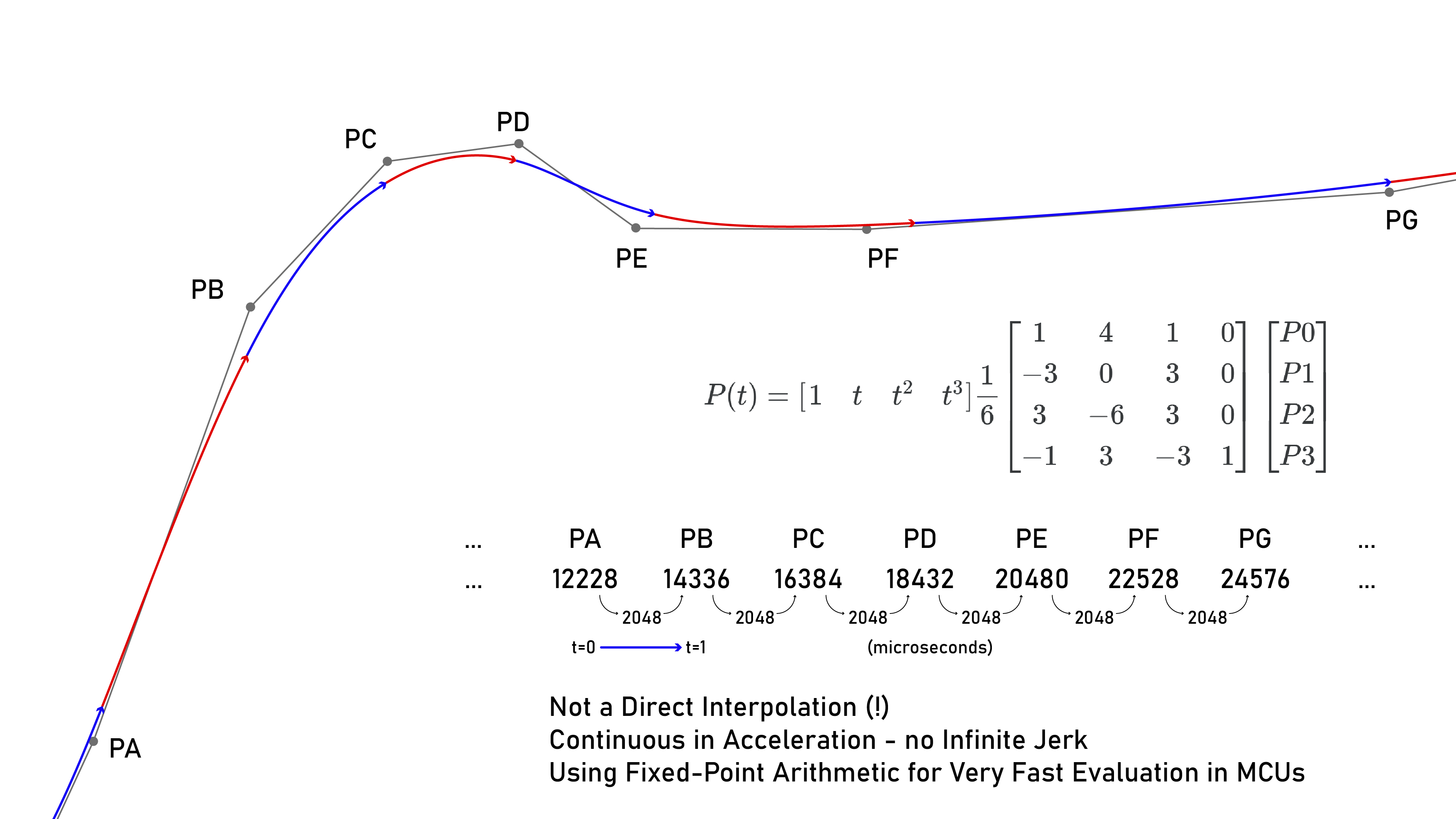

Fixed-Interval Basis Spline Segmentation
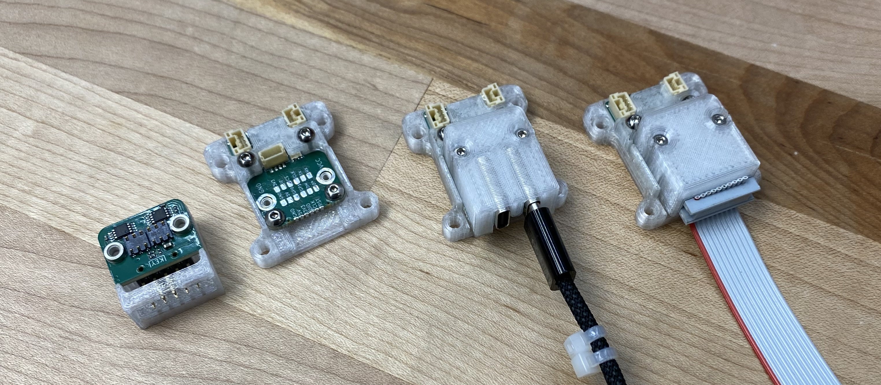
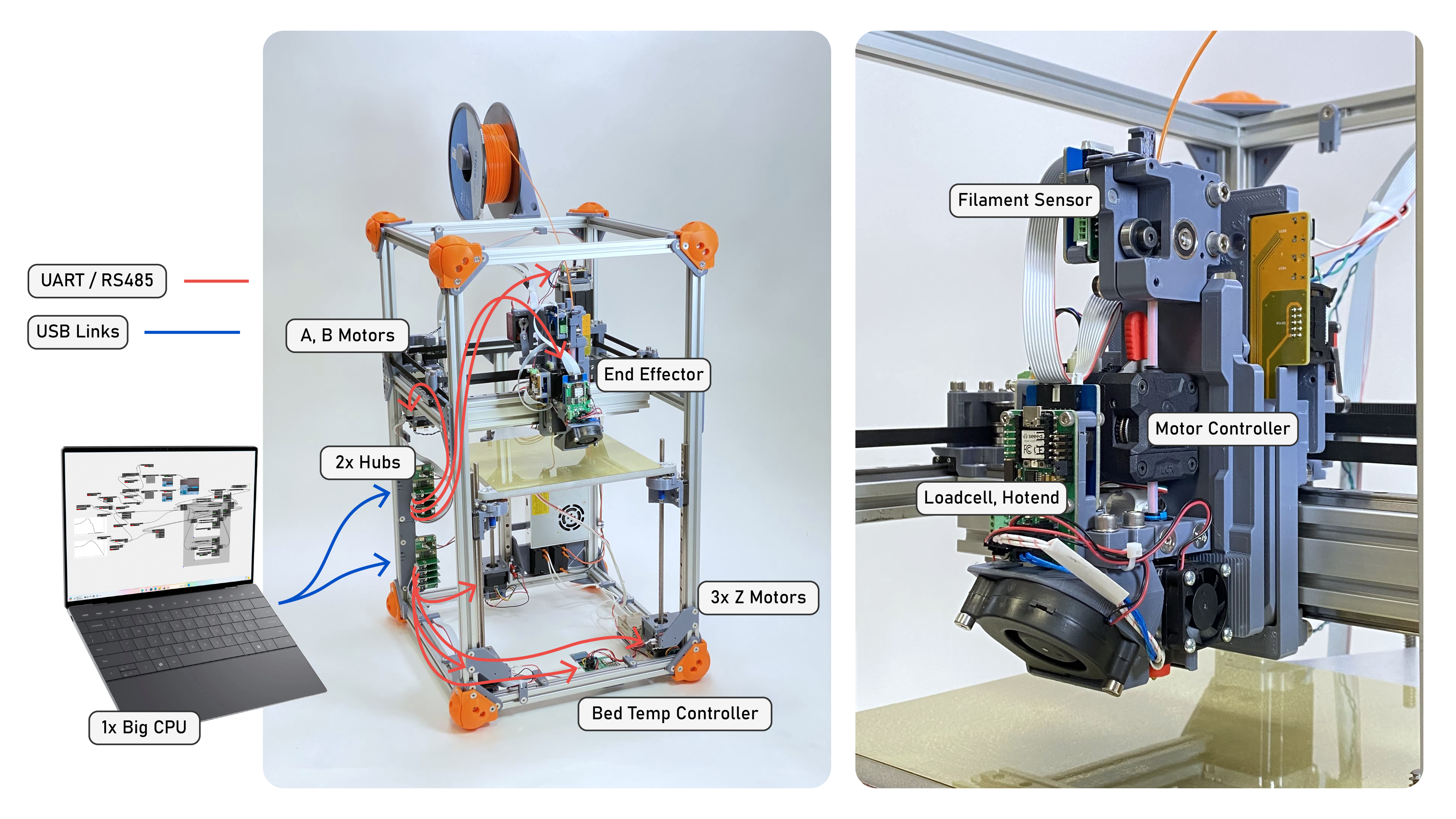
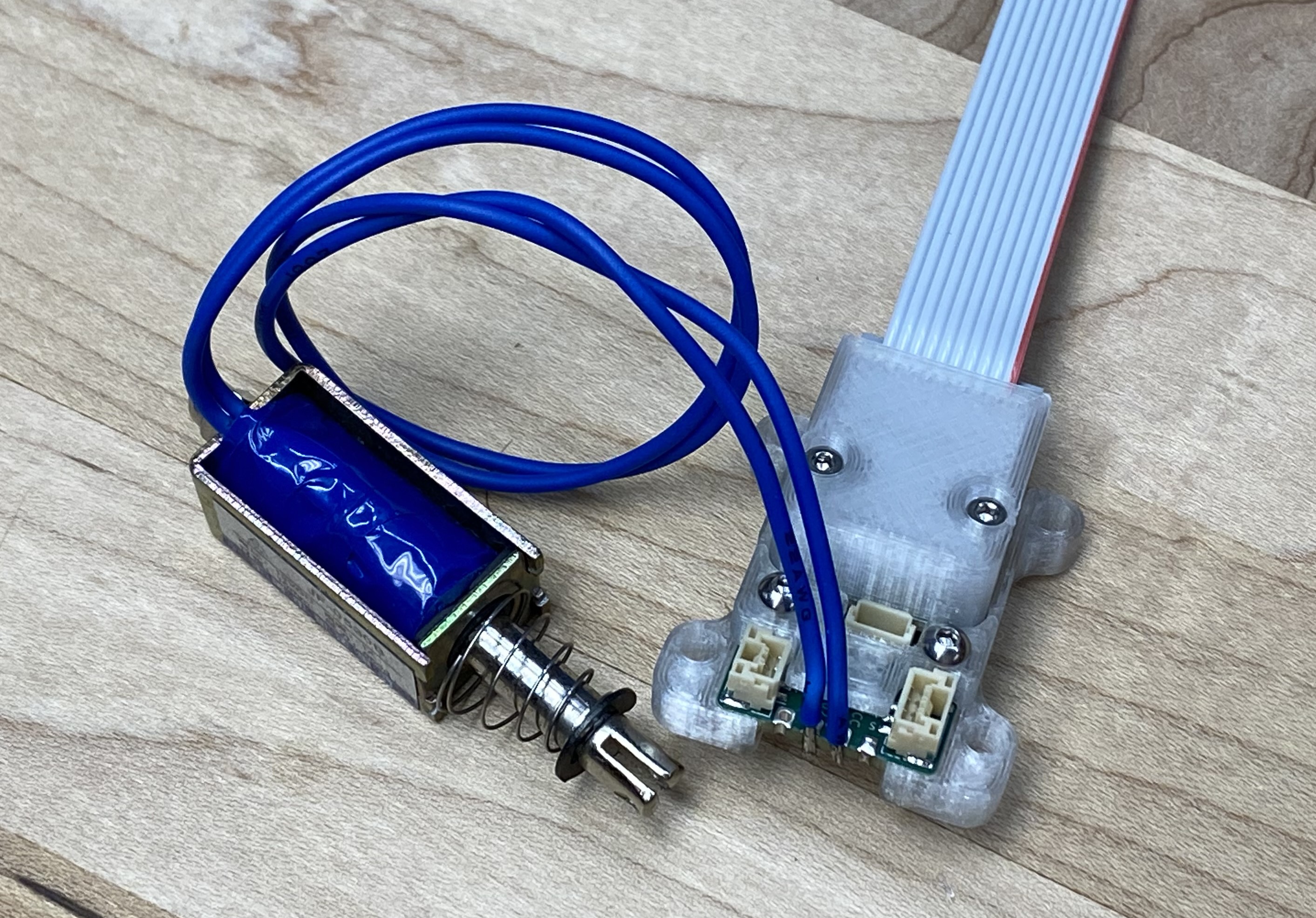
Swappable PHY's mean we can generalize modules across link layer technologies.
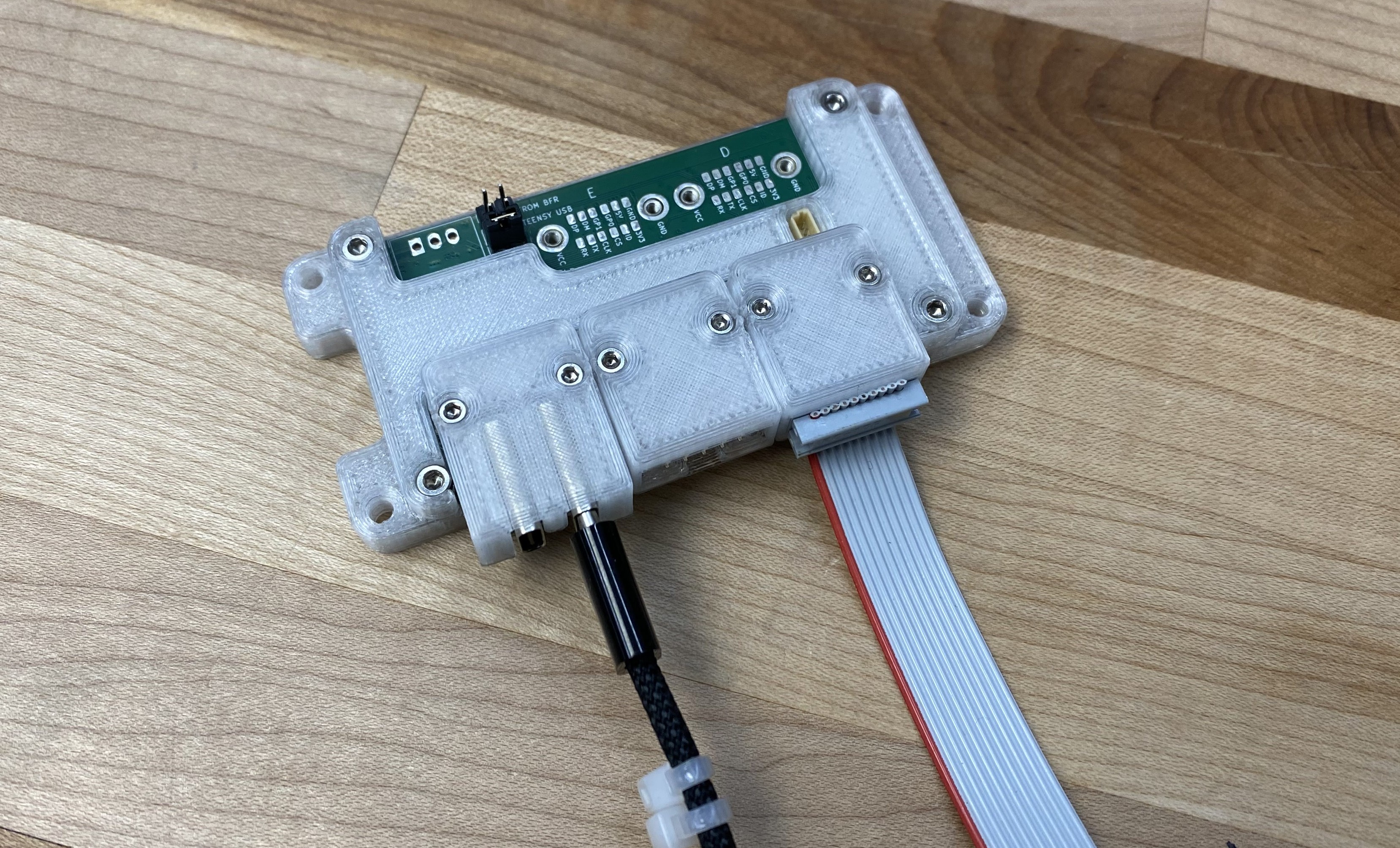
Hubs like this one let us assemble systems that span multiple link types.
Read, Jake Robert. Distributed dataflow machine controllers. Diss. Massachusetts Institute of
Technology, 2020.
mods.cba.mit.edu (Neil Gershenfeld + CBA), "Dynamic Toolchains" (Hannah Twigg-Smith, Nadya Peek)
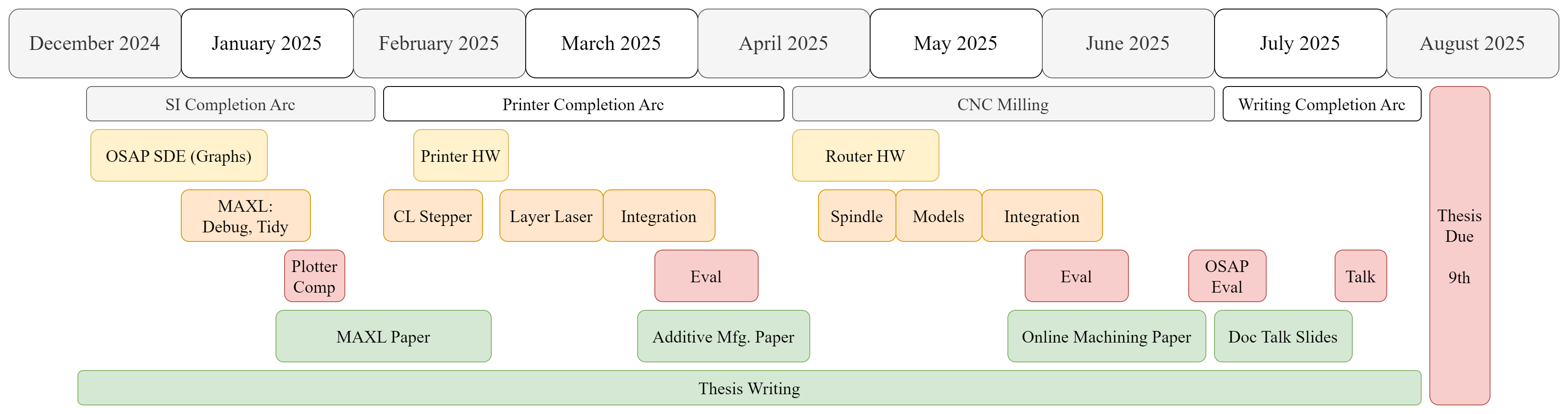
Printer Completion
Bring the optimizer online, and close the outer loop - improving models continuously.
Evaluate:
- Performance (speed, precision) vs. SOTA
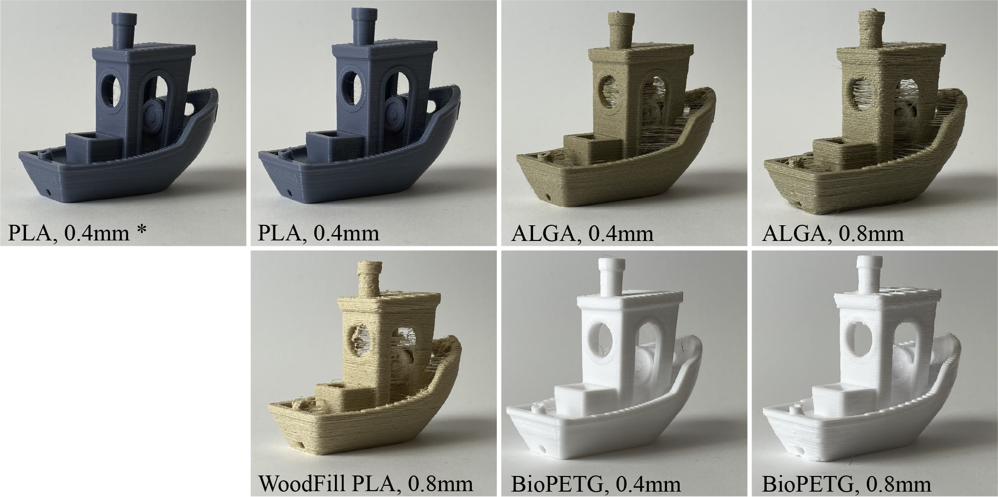
- Heterogeneity of materials.
- Number of parameters reduced.
- Performance (speed, precision) vs. SOTA
- Heterogeneity of materials.
- Number of parameters reduced.
CNC Machining
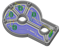
Develop cutting and resonance models, deploy them in real time.
Evaluate:
- Performance vs. SOTA
- Adaptability across Materials and Tools
- Number of parameters reduced.
- Performance vs. SOTA
- Adaptability across Materials and Tools
- Number of parameters reduced.
MAXL
Polish MAXL interfaces, run the Plotter Comp
Evaluate:
- Spline Lossiness
- Performance
- Heterogeneity of Kinematics
- Deployability
- Spline Lossiness
- Performance
- Heterogeneity of Kinematics
- Deployability
OSAP
Continue development, Evaluate!
Evaluate:
- Size and Time overhead
- Networking overhead
- Time sync precision and jitter
- Reliability
- Size and Time overhead
- Networking overhead
- Time sync precision and jitter
- Reliability
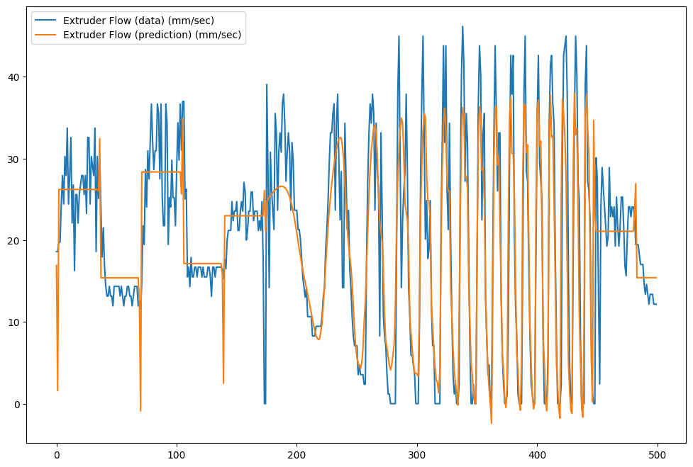
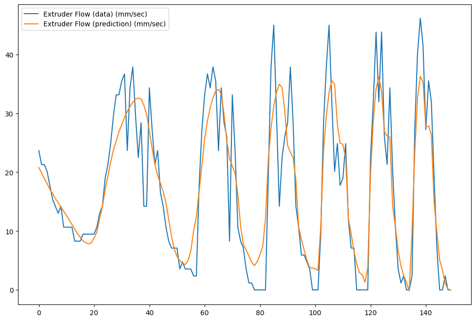
Simple MLP to fit flow, given extruder history.
W/ Yuval Mamana
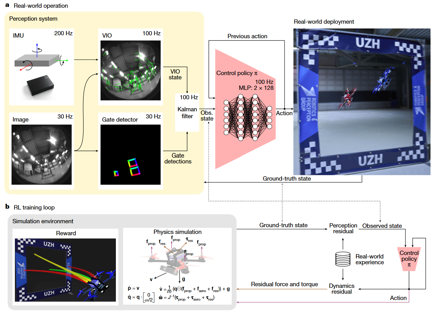
Kaufmann, Elia, et al. "Champion-level drone racing using deep reinforcement learning."
Nature 620.7976
(2023): 982-987.